1 Introduction

Switched Linear Systems (SLS) are hybrid dynamical systems whose dynamics are represented by a collection of Linear Systems (LS), together with an exogenous switching signal determining at each time instant the evolving LS. Hybrid systems capture the continuous and discrete interaction that appears in complex systems ranging from biological systems ¹⁴ to automotive systems ⁷. For SLS, many contributions have been reported concerning such basic system properties as stability, controllability, and observability.

Since the conditions for the observability with unknown inputs of the individual LS have been already established ⁴, the main problem for the observability of SLS is then to infer, from the knowledge of the continuous measurements, which LS is evolving. This is usually referred to as the distinguishability problem. This problem, together with the SLS observability, has been extensively studied in the literature for the case of known inputs ^1,9,13,18,20. However, the observability of continuous-time SLS subject to unknown disturbances and unknown switching signals has received less attention.

In the context of unknown switching signals, the concept of observability of SLS becomes more complex than in the LS case. The complexity arises from the two following reasons: first, because the autonomous case ²⁰ becomes non-equivalent to the non-autonomous case ^1,9,13, as the input plays a central role; second, because the unknown switching signal may make the system's trajectory to be observable even if it is evolving in a unobservable LS¹.

A geometric characterization of the main results presented in ^{1, 9, 13, 20} for SLS with unknown switching signal and no maximum dwell time was reported in a previous work ¹¹.

If on the contrary a maximum dwell time is considered, then the SLS state does not need to be recovered before the first switching time, but after a finite number of switches, either by taking advantage of the underlying discrete event system ⁹ or by investigating the distinguishability between LS ¹³. This problem has been considered in ⁸ for autonomous systems and in ⁹ and ¹³ for the known input case.

Concerning the observer design, if the switching signal is unknown then the observer for SLS requires to estimate the switching signal from the continuous measurements via a location observer. In ², the location observer uses a residual generator to infer a change in the continuous dynamics. In ¹⁰, an algorithm for computing the switching signal has been proposed for monovariable SLS with structured perturbations (i.e. disturbances with known derivatives). In ³, a super twisting based observer for unperturbed switched autonomous nonlinear systems has been presented. In ⁶, the location observer is formed by a set of Luenberger observers with an associated robust differentiator used to obtain the exact error signal which updates the estimate.

2 Preliminaries

2.2 Preliminaries on Linear Systems

The next lines review some of the basic geometric concepts on LS which are mainly taken from ²¹.

A Linear System (LS) is represented by the dynamic equation

1

where x ∈ X = ℝⁿ X = 1" is the state vector, 𝒰 ∈ = ℝ^g is the control input, y ∈ Y = ℝ ^q is the output signal, d ∈ D = ℝ ^m is the disturbance and A,B,C, and S are constant matrices of appropriate dimensions.

Throughout this work Σ(Α, Β, C, S) denotes the LS (1). When the matrices are clear from the context, a LS is simply denoted by Σ.

For an initial condition x(t₀) = x ₀, without disturbance (d(t) = 0), the solution of (1) is given by

2

The input function space, denoted by 𝒰 _f, is considered to be L _p (𝒰),¹ i.e. it contains piecewise continuous functions. Throughout the paper, Β stands for Im Β (image or column space of B), S for Im S and Κ for ker C (kernel or null-space of C).

A subspace Τ⊂ X is called Α-invariant if AT ⊂ T. The supremal Α-invariant subspace contained in Κ is N = ker (C A ^{i -1)}. The subspace N is known as the unobservable subspace of the LS Σ.

A subspace V ⊂ X is said to be (A, B)-invariant if there exists a state feedback u = Fx such that (A + BF)V ⊂ V or, equivalent, if AV ⊂ V + B. The set of maps F for which (A + BF)V ⊂ V holds is denoted as F(V).

The set of (A, B)-invariant subspaces contained in a subspace ℒ ⊂ X is denoted by ℑ(A, B; ℒ). This set is closed under addition, then it contains a supremal element ^{5), (21} denoted as sup ℑ (A, B; ℒ). Furthermore, sup ℑ (A,B; ℒ) can be computed with the following algorithm.

Algorithm 1. ^{( 5 ), ( 21 )} The subspace sup ℑ (A,B; ℒ) = V ^(k) where V ^(k) is the last term of the sequence

3

where the value of k ≤ n-1 is determined by the condition V ^(k+1) = V ^(k) .

Lemma 2. ⁵ Any state trajectory x(t), t ∈ [t₀, τ] of Σ belongs to a subspace ℒ ⊆ χ if and only if x(t ₀ ) ∈ ℒ and ẋ(t) ∈ ℒ almost everywhere in [t ₀ , τ [.

A LS is observable under unknown inputs iff a non-zero state trajectory producing a zero output does not exist. This is formally stated below.

Theorem 3. ^{( 5 )} Let Σ(Α,Β, C, S) be A LS. Then the LS Σ is observable under partially unknown inputs if and only if the sup ℑ (A, S; K) is trivial.

2.3 The Switched Linear System's Model

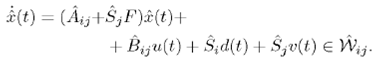
a SLS is described as a tuple Σ_σ = 〈ℱ,σ〉 where ℱ = {Σ_1;...,Σ _m } is a collection of LS and σ: [ t₀, ∞) → {1,..., m} is the switching signal determining, at each time instant, the evolving LS Σ_σ ∈ ℱ. The SLSs state equation is represented by

4

We use the notation x _i (t,x_ο,u[t_{0, τ}],d[t_{0, τ}]), to emphasize that the state trajectory x(t) is obtained when σ(t) = i and the inputs u(t), d(t) are applied since the initial condition is x(t ₀ ) = x ₀ . In a similar way, y _i (t,x ₀ ,u(t),d(t)) represents the output trajectory of xi(t,x ₀ ,u(t),d(t)), i.e.

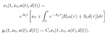
When we want to emphasize that the state trajectory is restricted to an interval [ τ_1; τ₂ ], we write y _i (t,x ₀ ,u _[ τ _1,u τ _2], d _[ τ _1,u τ _2] , where u _[ τ _1,u τ _2] , d _[ τ _1,u τ _2] are the restriction of the functions u(t), d(t) to [τ ₁ ,u τ ₂ ]. When d(t) = 0, we write y _i (t,x ₀ ,u(t)), and on autonomous systems we write y _i (t,x₀).

Let us remark that even though a SLS is formed by a collection of LS, the classical results on the fundamental properties of LS, such as stability, observability, and controllability, do not hold straightforwardly in the switching case.

2.5 Distinguishability in Perturbed Switched Linear Systems

In the following we review some of the results in observability using a geometric approach. This review is mainly taken from ¹¹, where it was shown that many observability notions arise in the perturbed case of SLS. Next, using the same framework of ¹¹, in Section 3 we will extend the results on a new (and less restrictive) observability notion that is more meaningful for the estimation using the proposed observer.

In the unknown switching signal setting, it is fundamental to infer the evolving linear system, and thus estimate the switching signal from the continuous input-output information. That problem is known as the distinguishability problem.

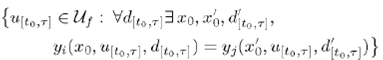
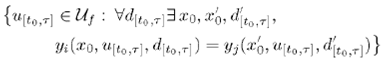
Formally, the LS Σ _i is said indistinguishable from another LS Σ _j if there exist x ₀ , d _{[ t0, τ ]} x' ₀ , and d' _{[ t0, τ ]} s.t.

5

If (5) holds for some x ₀ , d _{([ t0, τ ]} , x' ₀ , and d' _{[ t0, τ ]} , it is impossible to determine from the measured signals, u _{[ t0, τ ]} and y _{[ t0, τ ]} , if the state trajectory was generated by Σ _i or by Σ _j ·, consequently, it is impossible to determine if the continuous initial state is x₀ or x' ₀ . On the contrary, if (5) does not hold for all x ₀ , d _{[ t0, τ ]} , x' ₀ , and d' _{[ t0, τ ]} , then the pair of LS is said distinguishable, since it is possible to determine if the state is generated by Σ _i or by Σ_j from u _{[ t0, τ ]} and y _{[ t0, τ ])} . The indistinguishability subspace Ŵ _ij of Σ_i, Σ_j is defined as

and represents the set of initial conditions that under a particular input makes it impossible to determine which is the evolving system and the current discrete state. Then if the state trajectory x _i (t,x ₀ ,u _{[ t0, τ ]} ,d _{[ t0, τ ]} ) evolves inside 𝒬_iŴ _ij then it is impossible' to determine, from the measurements, if the evolving state trajectory is x _i (t, x₀, u _{[ t0, τ ]} , d _{[ t0, τ ]} ) or x _j (t, x´₀, u _{[ t0, τ ]} ,d' _{[ t0, τ ]} ), thus it is not possible to infer either the continuous initial state which could be x₀ or x' ₀ or the discrete state which could be σ(t) = i or σ (t) = j ∀t ∈ [ t0, τ ].

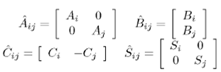
For a given pair of LS, Σ _i and Σ _j ·, the extended LS is defined as

6

The state space of is denoted by We denote by (t) the initial state, by the state trajectory, and by the disturbance signal of the extended LS .

Let us denote the natural projection of over X as 𝒬 _i : → X, i.e., 𝒬 _i ([x ^T x ^T ] ^T ) = x.

Lemma 4. Let Σ _i and Σ _j be two LS. Equation (5) holds if and only if the extended LS produces a zero output for all t ∈ [ t0, τ ], i.e. With =, u(t) and = [ dT (t) d'T (t) ]T.

Proof. The proof can be found in (¹¹). □

The following result characterizes the indistinguishability subspace.

Lemma 5. Let Σi and Σj be two LS and let Bij= [ Ŝ_ij]. Then the indistinguishability subspace Ŵ_ij is equal to the supremal -invariant subspace contained in = Ker ; denoted as sup ℑ

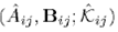
Proof. The proof can be found in (¹¹). □

By means of Algorithm 1 that computes (A, B)-invariant subspaces, the indistinguishability sub-space can be obtained. This subspace is fundamental, since the distinguishability and the observability can be derived from it.

It is worth noting that control inputs play a central role in inferring the evolving LS. In order to use such input to distinguish Σi from Σj·, these input has to be capable of steering the state trajectory outside 𝒬iŴij, i.e. the projection of the indistinguis hability subspace Ŵij over X. The conditions for this case are presented below.

Proposition 6. Let Σi and Σj be two LS. Then for almost every input Σi and Σj are distinguishable, i.e.

7

if and only if

. 8

Proof. The proof can be found in ¹¹. □

3 New Observability Conditions Meaningful in Practical Cases

In this section we derive less restrictive conditions for the distinguishability (hence, for the observability), that can be used in practical applications.

If condition (8) is not satisfied for a pair of LS Σ _i and Σ _j then, by Lemma 4, for every u(t) there exist ẋ ₀ and = [d(t) d'(t) ] ^T such that Σ _ij produces a zero output for all t ∈ [ t0, τ ]. As recalled in Subsection 2.2, an input that makes the extended system unobservable (equivalents Σ _i and Σ _j , indistinguishable) can be written as a state feedback = Fẋ, where F ∈ F(su_P ℑ ); Moreover, condition (8) gives the possibility for the input to be in Ŝij. Therefore, regardless of the input, we can write any disturbance making the LS Σi and Σj indistinguishable as = Fẋ + v(t), where v(t) ∈ Ŝ _ij . Now, by Lemma 2

This means that given u(t) there exists v(t) such that 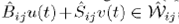in order to maintain the trajectory in the indistinguishable subspace Ŵ _ij .

Remark 7. Although the conditions of Proposition 8 guarantee that the control input can make the LS Σ_i and Σ _j distinguishable regardless of the disturbance applied, in general, if u(t) is discontinuous then the corresponding disturbance d and d', making Σ _i and Σ _j indistinguishable, must be discontinuous as well with discontinuities at the same time. However, since u(t) and d(t) (the control input and disturbance driving Σ _i ) are independent (in the sense that they are not functions of the same set of variables), the probability that their discontinuities are synchronized can be neglected.

A more convenient distinguishability notion for our setting (with less restrictive conditions), which can be derived using the same framework as in ¹¹, can be stated as the following problem.

Problem 8. (Distinguishability for almost every control input when u(t) and d(t) are independent, and the latter is continuous)

Assume that d(t) and d!(t) are continuous on t ∈ [ t0, τ ], under which conditions is

9

a shy set w.r.t _f ?

Notice than requiring d(t) and d'(t) to be continuous on t ∈ [ t0, τ ] is not a restriction over the class of disturbance that we consider in our setting, but rather it avoids the unlikely case where d(t) has discontinuities at the same time as u(t).

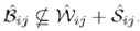
Lemma 9. Let Σ _i and Σ _j be two LS, and assume that d(t) and d'(t) are continuous on t ∈ [ t0, τ ]. Then

10

is a shy set, i.e. Σ _i and Σ _j are distinguishable for almost every input with u(t) and d(t) independent and d(t) continuous, if and only if either

11

or

12

holds, where Ŝ _i Im Ŝ _i and Ŝ _i = Im Ŝ _i with Ŝ _i = ∈ ℝ^2N and Ŝ _j = ∈ ℝ²ⁿ .

Proof. (Necessity) Assume that ⊆ Ŵ _ij and Ŝ _i ⊆ Ŵ _ij + Ŝ _j then by (11. Lemma 13), Ŵ _ij = sup ℑ Now let= d´(t)= Fẋ + υ With F ∈ F(su_P ℑ ); and u such that Ŝi d(i) + Ŝj u(t) ∈ Ŵij. Then notice that, if ẋ0 ∈ Ŵij and ẋ(t) Ŵij, thus by Lemma 2, ẋ(t) ∈ Ŵij regardless of u(t). Hence, (10) is equal to 𝒰f and (10) is not a shy set.

(Sufficiency) Assume that (10) is not a shy set. In (11) it was shown that if an input exists to distinguish two LS then almost every input can be used. Thus, (10) being a shy set implies that (10) is equal to 𝒰f i.e.

yi(x0,u [ t0, τ ], d[ t0, τ ] ) = yj(x´0,u[ t0, τ ], d´[ t0, τ ])

Let d'(t) = F+ υ (notice that if υ is continuous then d'(t) is continuous as well) with F ∈

F(sup ℑ ). Thus, by Lemma 2

13

In particular consider d(t) = 0. Since u(t) can be discontinuous on [ t ₀ , τ ] and d'(t) cannot, then evolves inside Ŵ _ij for every u(t)i.e. ⊆ Ŵ _ij . Now, consider d(t) ≠ 0. Since ( + Ŝ _j F) (𝑡) + evolves inside Ŵij, then (13) implies that for every d(t) there exists u(t) such that Ŝi d(t) + Ŝj u(t) ∈ Ŵij, i.e. Ŝi ⊆ Ŵij + Ŝj which completes the proof. □

Based on the distinguishability result we can state the observability for SLS.

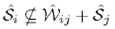
Theorem 10. Let 𝒢 = 〈ℱ, σ〉 be a SLS with partially unknown inputs and maximum dwell time τ = ∞. Then, the continuous state x0 and x(t) and the discrete state σ0 and σ(t) can be uniquely computed (said observable) for almost every control input, with u(t) and d(t) independent and d(t) continuous, if and only if every LS Σi ∈ ℱ is observable with partially unknown inputs (i.e. according to Theorem 3) and ∀Σi; Σj, ∈ ℱ i ≠ j, either ⊈ Ŵ _ij or Ŝ _i ⊈Ŵ _ij + Ŝ _j .

Proof. The proof follows from the previous argument. □

4 Observer Design for Perturbed SLS

In this section we show that if the continuous and the discrete states of the SLS are observable according to Theorem 10, then the SLS admits an observer based on a multi-observer structure, in which a finite-time observer is designed for each LS composing the SLS. It will be shown that, based on the observability results previously presented, a set of finite-time observers allow us to decide the evolving LS from the output estimation error. The observability of the SLS implies that the observer associated with the evolving /.Swill produce a zero output estimation error whereas the rest of the observers associated to LS that are distinguishable from the evolving one, cannot produce a zero output estimation error. Thus, the evolving LS is the one associated to the observer with zero output estimation error, whereas an exact estimation of the continuous state is provided by such observer. This observer extends the design proposed in ¹² in order to consider unknown inputs.

The construction of the observer for each LS is based on the multivariable observability form (see, for instance, ¹⁶⁾⁾. Let us firstly introduce some results about the transformation of an observable LS into such form.

Lemma 11. If the LS is observable under partially unknown inputs, i.e. if sup ℑ (A, S; K) is the trivial subspace, then there exists a set of integers {r₁,..., r _m } such that ∀ _i ∈ {1,..., m} ∀k ∈{0,...,r _i -2}, _Ci A ^k S = 0 and rank(0 _{ri... , _rm} ) = n where

Proof. The proof is presented in Appendix A. □

The values {r₁ ..., r _m } are known as the observability indices of ∑(A,B,C,S) ¹⁶. A LS observable under unknown inputs can be transformed by means of the similarity transformation T, defined such that T- ¹ = O_{r1..., _rm} , into the multivariate observability form² (see ^l6)).The resulting LS is given by the following matrices.

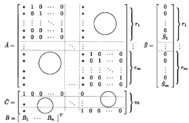
Notice that the transformed LS is composed of blocks, each one in the observer canonical form (see ¹⁶⁾⁾, but coupled only through the measured variables . Each i-th block is of dimension ri and is of the form

14

where the aji (y) j = l,...ri, is a linear combination of the output variables ... and

In what follows, let us consider the following assumption.

A. 5. The disturbances are differentiate and satisfy L _i ≥ with known constants Li, i = 1,... ,m.

Thus, we can add to (14) the dynamics of i.e.

Then, an observer based in the robust differentiator described in ¹⁷ can be designed for each block in order to estimate the state of the system in the presence of disturbances. The observer is designed in such a way that its error dynamics coincides with the differentiation error of ¹⁷, for which convergence has already been demonstrated in ¹⁷.

Thus, each block admits the following observer:

15

Defining the error dynamics as eji , = j= 1,..., m and = - ξ yields to

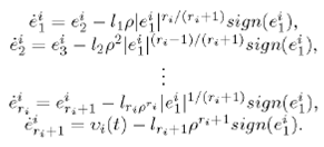16

Since the m subsystems are only coupled through the measured variables, which are fed into the observer by output injection through the terms aji (y), the error dynamics of the subsystems are independent from each other and coincide with the form of the differentiation error of the high order sliding mode differentiation presented in ¹⁷. Thus, with the proper choice of the observer parameters ρ and l _i a finite-time convergence to the continuous variables can be obtained in the presence of the disturbance d(t) ¹⁷ with arbitrary small convergence time. Thus, an estimation of the variables ,..., is obtained in finite-time. By designing an observer (15) for each block, the continuous state x(t) of the LS can be estimated in finite-time.

Finally, assuming that each pair of LS Σi and Σ _j is (u_[τ1,τ2] y _[τ1,τ2])-distinguishable under unknown inputs, if an observer is designed for each LS with time convergence bound τ < τ₁< τ₂, then the observer associated to the evolving LS will be the only one maintaining e _y (t) = y(t) - ỹ(t) = 0 ∀t ∈ [τ₁,τ₂] (unlike the known input case where the ξ variable would be also maintained at ξ = 0, in the unknown input case ξ ≠ 0 ¹²⁾⁾.

Lemma 12. Let Σ_σ(t) be a SLS and its observer with time convergence bound τ, and let σ(t) = i, ∀t ∈ [t ₀ ,t₂]. Then, if Σ _i and Σ _j are distinguishable under unknown inputs according to Lemma 9, then for almost every input u(t), eyj (t) ≠ 0 almost everywhere in [τ,t₁) (where eyj(t) is the output error signal e _y (t) = y - ỹ _j of the j-th observer).

Proof. The proof follows by noticing, from (15), that whenever the output error signal eyj satisfies eyj = 0, then the observer becomes a copy of its associated LS, driven by a perturbation signal ξ and producing the same output of Σ _i , because due to finite-time convergence of (15) the error correction terms in (15) associated to each block become equal to zero. However, as the Σ _i and Σ _j are distinguishable, then eyj = 0 cannot occur on a nonzero interval.

Thus, it follows by the assumption that Σ_i and Σ _j are distinguishable under unknown inputs that whenever σ(t) = i, ∀t ∈ [τ,t₁) only the observer associated to Σ _i satisfies eyi = 0 in the interval [τ,t₁)□

Hence, a multi-observer structure depicted in Fig. 1 can be used to estimate the continuous state x(t) of the SLS and to compute the switching signal σ (t). Notice that, since by Lemma 12 only the observer associated to the evolving LS gives e _y = 0, then by analysing this error signal the evolving LS can be ascertain. In a similar way, once the evolving LS Σ _j has been detected, the switching occurrence to another LS, say Σ _j , can be detected by the time when the error signal no longer satisfies e _y = 0, because by the pairwise distinguishability when switching from Σ _i to Σ _j the signal eyi can no longer be maintained zero from a nonzero interval.

Fig. 1 Observer for perturbed SLS 

Remark 13. Let Σ _i and Σ _j be two LS observable under unknown inputs. Suppose the distinguishability conditions of Proposition 6 do not hold but those of Lemma 9 hold. In such case, as pointed out in Remark 7, if we make u(t) discontinuous then two cases may occur. The first one, no disturbance exists in Σ _j such that (5) holds, in which case by Lemma 12 only the output estimation error of the observer associated to Σ _i will be zero. The second one, the disturbance in Σ _j required to make Σ _i and Σ _i indistinguishable is discontinuous as well, in which case the observer associated to Σ ₀ may estimate x'(t) and d'(t) such that (5) holds, but the discontinuities of d'(t) will be synchronized with those of u(t) with a transient with e _y ≠ 0. However, since u(t) and d(t) are independent then the synchronization of their discontinuities given by the observer associated to Σ _j are identified as unlikely, thus discarding Σ₅· as the evolving system. In this way discontinuous inputs in U _p , are useful to make the LS distinguishable and the evolving LS can be inferred from the observers' output estimation error.

Proposition 14. Let the continuous and discrete state of Σ _σ(x) be observable under unknown inputs, i.e. each LS Σ _i ∈ℱ is observable under unknown inputs and pairwise the LS in ℱ are distinguishable under unknown inputs, and let T _k be the similarity transformation taking the LS Σ _k into the multivariate observer form. Then the state x(t) of Σ _σ{x) and the switching signal σ(x) can be estimated by the following procedure:

Proof. The proof follows by the previous argument and from the observability result which requires each pair of LS to be distinguishable for almost every control input. □

5 Illustrative Examples and Simulations

Example 15. (Observability under unknown inputs)

Consider the perturbed SLS Σ_σ(t) where σ(t) is an exogenous switching signal and ℱ = {Σ_ι, Σ₂} is the continuous dynamics composed of LS with system matrices as in Table 1, input matrices Β ₁ = [0 2 0 ]^T and B ₂ = [ 0 1 1 ] ^T , output matrices C₁ = [ 0 0 1 ] and C ₂ = [ 0 1 -l ], and disturbance matrices S₁ = [ l 0 0 ]^T and S₂ = [ 1 0 0 ]^T.

Table 1 System matrix of linear systems 

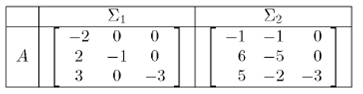
The indistinguishability subspace of Σ₁ and Σ₂ is

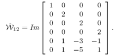
Since Ŵ ₁₂ is not trivial for every x ₀ ∈ 𝒬₁Ŵ ₁₂ = X, there exist u(t) and d(t) such that (5) holds for some x' ₀ and d'(t), making it impossible to infer the evolving LS.

For instance, suppose that the evolving LS is Σ₁, with

x ₀ = [ 0 2 0] ^T , u(t) = 43 e^-3t + 23

and d(t) = 0, then the output is

y _i (t,x ₀ , u(t),d(t)) = 43 e^-3t + 23,

since the LS Σ _j produces this same output with

x´₀ = [ 0 1 1 ]^T , u(t) = 43 e^-3t + 23

and

d´(t) = - 209 + 389 e^-3t- 163 te^-3t,

then it is impossible to determine, from the input-output behavior, the evolving LS and the continuous initial state for the current state trajectory. Hence, the LS Σ₁ and Σ₂ cannot be distinguished for every state trajectory.

Moreover, since ⊂ Ŵ ₁₂ , then according to Proposition 6, there is no input u(t) allowing to distinguish Σ₁ from Σ₂, i.e. the effect of the input u(t) does not show up at the output of the extended system.

Furthermore, since ⊂ Ŵ ₁₂ + and 𝒬₁Ŵ ₁₂ = X then for every state trajectory of Σ _i , there exists a state trajectory of Σ₂ producing the same output, therefore it is always impossible to distinguish the LS Σ₁ from the LS Σ₂, i.e. ∀x ₀ , u(t), d(t) ∃ x' ₀ ,d'(t) such that (5) holds, in fact with x'o such that ∈ Ŵ ₁₂ and d´(t) - F(t) such that F ∈ F(Ŵ ₁₂ ) (e.g. F = [ 1 - 4 4 0 2 0]), then (5) holds.

The existence of this state feedback implies that for every state trajectory of the LS Σ₁, there exist x' ₀ and d'(t) (not necessarily constructed as a state feedback) in Σ₂ such that it is impossible to determine the evolving system and the initial continuous state since there exist state trajectories in both LS producing the same input-output information.

Example 16. (Observability and Observer Design)

Now, if we consider the SLS composed of LS with system matrices as in Table 1, input matrices Β ₁ =[ 1 2 0 ]^T and B₂ = [ 0 1 0]^T , output matrices C₁ = [ 0 0 1 [ and C ₂ = [ 0 1 -1], and disturbance matrices S _{l =} [ 1 0 0 [ ^T and S₂ = [ 1 - 12 - 12 ] ^T , then the indistinguishability subspace Ŵ ₁₂ is

It is easy to verify that, both Σ₁ and Σ₂ are observable under unknown inputs, in addition, Σι and Σ₂ are distinguishable from each other according to Lemma 9 as ⊈ Ŵ ₁₂ . Thus, according to Theorem 10, the continuous and discrete states of the SLS Σ_σ(t) are observable, in infinitesimal time, for almost every control input u(t), and the proposed observer design can be applied to estimate the continuous and discrete states of Σ_σ(t).

Fig. 2 illustrates the application of Lemma 12 to infer the evolving LS. It can be seen that the output estimation error e 1y, related to the observer of Σ₁, converges to zero in finite-time, whereas the output estimation error e 2y, related to the observer of Σ₂, cannot be zero (when the system evolves in Σ₁ for a nonzero interval, allowing to infer the evolving LS and the discrete state σ. In this example, the detection of the switching time is trivial, as the continuous output is discontinuous. At the switching instants, the observers are reinitialized as described in Proposition 14. After the reinitialization at 3.5s, only the output estimation error of the observer associated to the evolving LS can be maintained as zero, in this case the signal, ey2 is the only one that remains at zero.

Fig. 2 Inferring the evolving LS from the output estimation error 

Hence, the proposed observer determines the evolving LS and the switching signal using only the output information y(t) in spite of the unknown disturbance affecting the system.

Fig. 3 shows the estimation of the continuous state using the procedure described in Proposition 14. The continuous and discrete states of the SLS are estimated in finite-time by the proposed observer, using only the output information y(t) in spite of the unknown disturbance d(t).

Fig. 3 Estimation of the continuous state x(t) 

It is worth noticing that, in the case where the disturbance is scalar, the proposed observer also estimates the unknown disturbance d(t). However, in general, the unknown disturbance is not estimated. The design of an unknown input observer for SLS can be derived straightforwardly if in addition to the observability under unknown inputs we require each LS to be invertible (i.e. two different disturbance signals cannot produce the same output).

6 Conclusions

Necessary and sufficient conditions for a new observability notion for perturbed SLS, meaningful for practical applications, have been derived, which result in less restrictive conditions than those reported previously in the literature. Based on the observability analysis we derive the conditions for detecting the evolving LS and estimating its continuous state from a collection of finite-time observers in spite of the acting disturbance.

As future work, we consider to model the discrete dynamic by Petri nets to reconstruct the continuous and discrete states after a finite number of switching.

A Proof of Lemma 11

Proof. The proof follows a similar development as the one shown in (5, Section 4.3.1). Consider the following iterative process, for simplicity let Β = 0 as the control input does not affect the observability under unknown inputs in LS. Let

17

with _qo (t) = y(t) and y₀ = C. Differentiating (17) yields = Y ₀ Ax(t) + Y ₀ Sd(t). Let P₀ be a projection matrix such that kerP₀ = Im(y₀S'). Thus

18

Let and Y₁ = then (17) and (18) can be combined to get _qi (t) Y _lx (t). It is easy to see that

The k-th iteration of the procedure yields q _k (t) Y _k x(t) such that

Notice that such iteration process coincides with Algorithm 1 and therefore converges to sup ℑ(A,S;K). Reordering Y _k yields the matrix 0 _{{r1,... rm}} . Since, after a sufficient number of iterations k, kev Y _k = sup ℑ (A,S;K.) = 0, then rank (0_{ri..._irm}) = n. □