


 nueva página del texto (beta)
 Inglés (pdf)
 Artículo en XML
 Referencias del artículo
 Enviar artículo por email
 Citado por SciELO
  Similares en
SciELO
Similares en
SciELO 
 Permalink
1. Introduction
Man-made pollution of the atmosphere, hydrosphere, pedosphere, and biosphere has grown in recent years. According to the World Health Organization (WHO), 92% of the world’s present population lives in places where air quality is worse than the limits set by the WHO (2016). Therefore, monitoring pollution levels especially in urban areas, where more than half of the world’s population lives, is of utmost importance. Anthropogenic particulate matter (PM) accounts for about 10% of the total global aerosol amount, but with large regional differences (Perrino et al., 2010). The dangers posed by pollutants to health, the environmental system, and the atmospheric radiation budget have been shown in numerous studies (e.g., Pope III et al., 1992; Luo et al., 2012; Maher et al., 2016; Salmani-Ghabeshi et al., 2016; Song et al., 2016; Bourliva et al., 2017; Cao, 2017). Current investigations focus on the identification of highly polluted areas through direct monitoring, (bio)magnetic monitoring, backward modeling of sources and pathways of pollutant agents, and forecasts of high-pollution events.
Direct geochemical monitoring is often time-consuming, laborious, and costly, whereas magnetic methods are fast and inexpensive (Petrovský and Ellwood, 1999). Magnetic methods identify the amount, concentration, type, and grain sizes of iron oxides, iron hydroxides, and sulphides that are linked to heavy metals. Furthermore, magnetic techniques have shown to be capable of discriminating between different sources of pollution (e.g., Hoffmann et al., 1999, Hansard et al., 2012; Zhang et al., 2012;). Specifically, biomagnetic monitoring uses magnetic methods to identify ferromagnetic (s.l.) PM captured by biological matrices.
Already in 1926, Gustav Ising studied environmental processes in a glacial setting using magnetic minerals (Maher, 2007). In his pioneering work he measured magnetic susceptibility and natural magnetic remanence of annually laminated lake sediments from Sweden. He found that the magnetic properties of the sediments varied seasonally and with distance from their ice margin source (Maher, 2007). Thompson formally defined environmental magnetism as a discipline in the 1980s (Thompson et al., 1980). The materials investigated in environmental studies include soils, sediments, dust, rocks, organic tissues, and manmade materials. The magnetic properties of the different materials are used as proxies, for example, for provenance analysis of sedimentary basins, pollution assessment, and paleoclimate studies (Dekkers, 1997). The matrices used to investigate pollution in urban areas are predominantly soils and sediments, which act as long-term archives of pollution; urban dust taken from streets; plants and other surfaces; and airborne particles from air filters.
The close relationship between ferromagnetic (s.l.) minerals and heavy metals and other pollutants has been shown by combined analyses of chemical and magnetic data (Hanesch et al., 2007; Aguilar Reyes et al., 2012; 2013; Cejudo-Ruíz et al., 2015). Hazardous particles can be traced with magnetic minerals, because the latter are able to incorporate heavy metals in their structure (Scoullos et al., 1979; Oldfield and Scoullos, 1984; Thompson and Oldfield, 1986; Flanders, 1994; Matzka and Maher, 1999). For example, industrially derived magnetic minerals share an origin and existence with heavy metals and thus can be used as tracers of pollution (e.g.,Scholger, 1998; Evans and Heller, 2003). Heavy metals can be absorbed, adsorbed, or incorporated in the structure of magnetic minerals. For example, Mn, Ni, and Co can be incorporated directly into the structure of goethite (Cornell, 1991). Georgeaud et al. (1997) reported that magnetite is a possible carrier of heavy metals such as Pb, Cd, Cr, or Ni. Particles finer in size than 10 µm-called PM10-have a high specific surface, which makes these particles efficient carriers of pollutants such as heavy metals and polycyclic aromatic hydrocarbons (PAH) (Hoffmann et al., 1999; Lu et al., 2011). Laboratory studies of iron oxides in redbeds revealed that these particles are highly adsorbent of heavy metals (Rose and Bianchi-Mosquera, 1993).
Most commonly, measurements of magnetic susceptibility and isothermal remanent magnetization are used as proxy methods for the accumulation of heavy metals. However, heavy metals are not equally well correlated with these magnetic parameters. Soils, sediments and dusts contain a complex natural mixture of magnetic minerals of different grain sizes (Hoffmann et al., 1999). Therefore, it is necessary separating the anthropogenic magnetic signal from its natural background (Hoffmann et al., 1999; Yang et al., 2015). However, the approaches used so far are diverse and approximate, which makes a comparison between different studies difficult.
The aim of this review focuses on biomagnetic monitoring of ferromagnetic (s.l.) minerals used as tracers for pollutants, including its advances and current weaknesses. First, the pollutants found in the pedo-, hydro-, bio-, and atmosphere are presented, including their harm to humans and the ecosystem. This is followed by an introduction of the ferromagnetic tracer minerals, their detection and the implications of the magnetic parameters. Subsequently, a thorough review of current advances of biomagnetic monitoring of anthropogenic pollution in urban centers is presented, followed by an outlook on future environmental studies. Finally, conclusions are drawn about the current state of research.
2. Pollutants, their pathways and matrices
Primary pollutants, such as heavy metals that derive from natural or anthropogenic sources, are discharged directly into the troposphere (Smith, 1990). Dust containing heavy metals is dispersed globally by atmospheric circulation and becomes a significant component of sediments, soils, biosphere, and hydrosphere. The most common heavy metals of anthropogenic origin have a variety of sources, including vehicular and industrial combustion, heating, and abrasion processes. In recent years, man-made iron oxides from combustion of fossil fuel, particles caused by the wear of roads and tires, metal smelting, production of cement, coal burning power plants or steel manufacture, and agricultural processes have made their way into the environmental system (Thompson and Oldfield, 1986; Evans and Heller, 2003). Elements such as Pb originate from leaded gasoline, whereas Cu, Zn, and Cd derive from car components, abrasion of tires, lubricants, and industrial or incinerator emissions. The corrosion of cars and the chrome plating of vehicle parts free particles Ni and Cr; and As stems from emissions of fossil fuel combustion, from industrial activities, and from the use of pesticides and pigments (Zhang et al., 2012).
Iron oxides are among the most omnipresent components of natural materials, accounting for about 2% of Earth’s crust. They form part of natural processes in the lithosphere that involve large-scale and long-term material movement, mountain building, sea-floor spreading, and rock weathering. Further sources of iron oxides are the eruption and flow of lavas, dispersal of volcanic ashes, and transport of eroded sediments (Figure 1; e.g., Thompson and Oldfield, 1986). A small and generally insignificant amount of iron oxides arrives as cosmic flux.

These natural and anthropogenic magnetic minerals reach the atmosphere as fly ash. They remain there for weeks or months and can be transported for hundreds to thousands of kilometers (Evans and Heller, 2003; Johansson et al., 2007). The amount of magnetic material deposited per unit of surface area varies inversely with the distance from the source. A general assumption is that a rough equilibrium is maintained between particles washed away and new ones deposited (Evans and Heller, 2003). Typically, at 1 km from the source, the amount of magnetic material is 1 µg/cm2 (Evans and Heller, 2003).
Dry and wet deposition causes particles to reach the hydro-, bio-, and pedosphere (Petrovský and Ellwood, 1999). Dry deposition is the direct incorporation of particles in soil, in the hydrosphere, in vegetation, and on man-made surfaces, while wet deposition is the absorption of atmospheric pollutants into droplets followed by droplet precipitation or deposition on Earth’s surface (e.g., rain droplets in fog) (Zannetti, 1990). In the hydrosphere, particles accumulate as sediments in rivers, lakes, and oceans. In the pedosphere, particles are incorporated in top soils or accumulate on surfaces. Finally, particles can be resuspended in the atmosphere by wind erosion and sea spray.
2.1. ATMOSPHERIC POLLUTION-AIRBORNE PARTICLES
Airborne particulate matter (PM) is, besides ozone (smog), nitrogen oxides (NOx), sulfur oxides (SOx), or, specifically, SO2, carbon monoxide (CO), and lead (Pb), a pollutant for which the Environmental Protection Agency has established air quality standards (Esworthy, 2013). Volatile organic compounds, e.g., PAH, are also counted in the classic pollutants (Holgate et al., 1999). Particulate matter is a mixture composed of solid and liquid particles, both of natural and anthropogenic origin, having diverse chemical and physical characteristics. Particles are classified by their aerodynamic diameter, because it determines transport, removal and deposition processes in the air and on Earth, and pathways within the respiratory tract of the human body (Kim et al., 2015). The typical grain size range for PM covers a few nm to tens of mm. PM is generally separated into (1) coarse particles, smaller than 10 μm in aerodynamic diameter (PM10); (2) fine particles, smaller than 2.5 μm (PM2.5); and (3) ultrafine particles, which are finer than 0.1 μm (PM0.1) (Sioutas et al., 2005; Hinds, 1999; Figure 2).
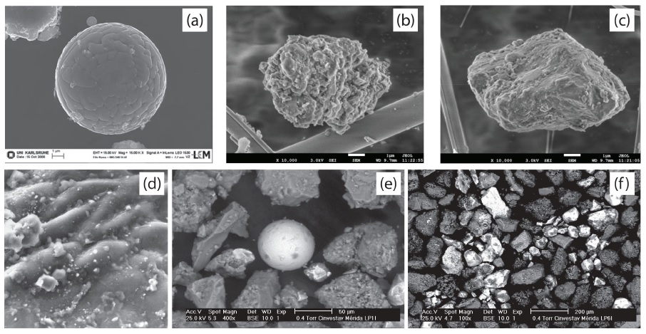
Figure 2 Scanning electron microscope images of anthropogenic particles. (a) Iron oxide fly ash (reproduced from Schleicher et al., 2010, with permission from The Royal Society of Chemistry). (b) PM10 soot particles (reproduced from Wu et al., 2015, licensed under CC-BY-4.0, http://www.mdpi.com/2073-4433/6/8/1195/htm). (c) PM2.5 soil dust particle (reproduced from Wu et al., 2015, licensed under CC-BY-4.0, http://www.mdpi.com/2073-4433/6/8/1195/htm). (d) Dust on roadside tree (photo by J. Matzka in Maher and Thompson, 1999, with permission from Cambridge University Press 1999; width of micrograph is 60 μT). (e-f) Urban dust. Spherical and luminous particles are coming from combustion processes and are mainly magnetite (photos by F. Bautista).
PM10 are inhalable particles that penetrate into the trachea, bronchi, and deep lungs (Figures 2b and 3). These particles often correlated with dust originating from paved roads, dirt roads, sites under construction and demolition, mining, industrial processes, agricultural operations and biomass burning. (Esworthy, 2013). PM10 are to a large part mechanically formed by the breakup of larger solid particles, but they also form during combustion processes, such as airborne wastes from industrial processes and motor vehicles (e.g., WHO, 2013, p. 8).
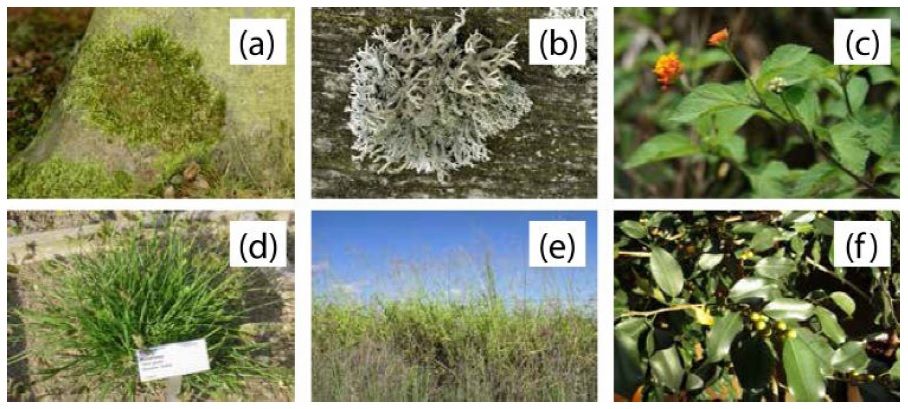
Figure 3 (a) Example of Hypnum cupressiforme and (b) Pseudevernia furfuracea, both by James K. Lindsey (http://www.commanster.eu/commanster.html) is licensed under CC-BY-SA 3.0. (c) Lantana camara by Franz Xaver (https://commons.wikimedia.org/wiki/User:Franz_ Xaver) is licensed under CC-BY-SA 3.0. (d) Eleusine indica by Daderot (https://commons.wikimedia.org/wiki/User:Daderot) is licensed under the public domain. (e) Panicum maximum by Harry Rose (https://www.flickr.com/photos/macleaygrassman/25136714676/) is licensed under CC-BY-2.0. (f) Ficus benjamina by PauliHartmut is licensed under the public domain.
PM2.5 is emitted directly from vehicles, smokestacks, and fires but can also form in reactions in the atmosphere from gaseous precursors, including sulfur oxides, nitrogen oxides, and volatile organics. These precursors occur naturally or in emissions from gasoline and diesel engine exhaust, and in emission from utility and other industrial processes (Esworthy, 2013; Figure 2c). Blanchard (2004) identified the composition of PM2.5 in various sites in the United States, Canada, and Mexico as sulfates, nitrates, ammonium, black and organic carbon, soil, and other particles such as trace metals from fossil fuel combustion and natural bioaerosols. It has been estimated that global emission of PM2.5 is composed half from natural and half from anthropogenic sources (Davidson et al., 2005).
Particles smaller than a micrometer mainly form through the condensation of metals or organic compounds that are vaporized in high-temperature combustion processes, and by the condensation of gases that have been converted to low-vapor-pressure substances by chemical reactions in the atmosphere (WHO, 2000, Chapter 7.3). The even-smaller PM0.1 consists of primary combustion products from vehicles, particularly from diesel and automobile exhaust, and includes organic compounds, elemental carbon, and metals (Sioutas et al., 2005).
Particles are further categorized through their origin. Primary PM can originate from natural processes such as aeolian dust, volcanoes, forest fires, living vegetation, and sea spray. Anthropogenic (magnetic) primary PM has its source in fossil fuels (coal and oil combustion in power plants, domestic heating systems, vehicle motors), the abrasion and corrosion of metallic parts (i.e., brakes), the erosion of asphalt roads, iron and steel manufacturing, and agriculture and waste processing plants (WHO, 2013, p. 4). Secondary PM (i.e., ammonium sulphate and nitrate, or sulphuric acids and nitric acids) is formed in the atmosphere and is generally found in small PM (WHO, 2013, p. 3).
Automobile traffic, as a main source of PM2.5 and ultrafine particles in urban sites, has an estimated contribution to PM2.5 of up to 50% (De Kok et al., 2006). Road transport can be seen as the single most important source of PM0.1 (Holgate et al., 1999). Pavement abrasion is rich in minerals containing Si, Al, K, Na, and Ca (Lindbom et al., 2006). Brake and tire particles can contain Cu, Sb, Pb, Cd, and Zn (Hjortenkrans et al., 2006). Further pollution-causing sources are direct-exhaust emissions, and iron particles, probably due to carbody rusting also ablation from the exhaust system (Petrovský and Ellwood, 1999). Particles deposited close to the edge of the roads are primarily non-spherical or angular. These particles are of localized significance: beyond distances of 20-30 m, vehicle-derived particles are usually negligible. Inside the roadside band, however, all living beings are exposed to higher concentrations of respirable particles (Petrovský and Ellwood, 1999).
Large amounts of heavy metals are found in fly ashes emitted from coal-burning power plants and industrial smelters (e.g., Petrovský and Ellwood, 1999; Szuszkiewicz et al., 2015). Heavy metals like As, Cd, Zn, and Pb, and probably also Br, Cr, and Mn, enrich most fly ash and are associated with small respirable particles (Maher and Thompson, 1999). Industrial fly ash also contains iron oxides such as magnetite and hematite. Magnetite and hematite, as well as maghemite, limonite, and magnesioferrite can be primary minerals. However, magnetite and hematite are formed mainly during the burning process in power plants through the oxidation of pyrite, marcasite, and siderite, but also ankerite and jarosite (Vassilev and Vassilev, 1996; Evans and Heller, 2003). Before being burned, coal is essentially non-magnetic. The combustion causes pyrite to dissociate and form pyrrhotite and sulfur gas. Above 1077 ºC pyrrhotite decomposes into sulfur and iron. In this process spherical iron particles of about 20 µm in diameter are formed and subsequently oxidize to magnetite (Evans and Heller, 2003). On average, 16% of coal burned in a power station becomes ash and about 16% of this ash is magnetic. In general, the particle size distribution of the burned coal fly ash is defined by the size of the pulverized coal and the temperature of combustion (Flanders, 1999). Furthermore, magnetite and hematite are produced during combustion from clay containing iron in coal through the growth of molten crystals, the reduction of Fe oxide by carbon and hydrogen, and Fe hydroxides dehydroxylation (Vassilev and Vassilev, 1996; Kapička et al., 1999). The processing of steel and the production of cement are further sources of iron oxide minerals (Petrovský and Ellwood, 1999). Cd, Cu, Pb, Zn, Cr, and Ni are derived from traffic and industrial emissions, mining, sewage sludge, pesticides, and fertilizers (Wei and Yang, 2010). Magnetite in fly ash in general appears as discrete rounded grains with a diameter between 1 and 10 µm, or as dendrites and octahedra in the glass (Petrovský and Ellwood, 1999). Hematite has been found as platy specularite or lamellar crystals, often forming rose-like shapes (Petrovský and Ellwood, 1999). The combustion of fossil fuel raises the concentration of magnetite from 10 ppm in the unburnt fuel to 500-10000 ppm in the combusted fuel; in the case of coal ash the magnetite content may rise up to 160000 ppm (Petrovský and Ellwood, 1999). Coal-fired fly ashes are rich in magnetite with grain sizes ranging from small single domain (SD) to large multidomain (MD) grains, with the largest grain size fraction from 2 to 50 µm. Magnetite mostly occurs as spherules, sometimes with an “orange peel” surface (Petrovský and Ellwood, 1999; Yang et al., 2007).
2.2. PLANTS, MOSSES, AND LICHENS AS RECEPTORS FOR POLLUTANTS
Tree leaves are considered efficient PM receptors and provide the potential for a large number of samples (e.g., Flanders, 1994; Mitchell et al., 2010; Rai, 2013). Leaves of deciduous species are used for short-term monitoring of PM pollution in urban areas (Matzka and Maher, 1999; Jordanova et al., 2010; Mitchell et al., 2010; Kardel et al., 2011; Hansard et al., 2012; Sadeghian, 2012; Sant’Ovaia et al., 2012; Hofman et al., 2017;), while evergreen species are suitable for longer-term monitoring (e.g., 1-3 years) depending on the leaves’ or needles’ life-span (Moreno et al., 2003; Urbat et al., 2004). Tree-trunk cores are used for historical or long-term PM monitoring (Zhang et al., 2008; Vezzola et al., 2017).
Kardel et al., (2011) found that deposition of PM on leaves mainly depends on leaf surface area and its surface characteristics. Certain morphological leaf characteristics such as surface roughness due to veins or rugosity and the presence of stellate trichomes favor deposition of PM. Trichomes increase the surface on which atmospheric particles can be deposited, and capture particles from air flowing along the leaf surface (Kardel et al., 2011). Furthermore, ridged, hairy leaves exhibit the greatest deposition capacity (Mitchell et al., 2010). Leonard et al. (2016) investigated PM loads on 16 common native plant species along Sidney roadsides and linked them to their leaf traits such as leaf area, shape, arrangements, as well as the presence of leaf hair. They found that leaves that are broadest below the middle (lanceolate shaped) accumulate more PM than leaves that are narrowest below the middle (obovate and elliptic shaped). Furthermore, they confirmed that plants with leaf hairs accumulated significantly more PM than plants without leaf hairs. Leonard et al. (2016) pointed out that some leaf traits might cancel themselves out in terms of PM capturing capacities. Therefore, the combination of different traits has to be taken into account. Hummock-forming plants that are found in peat bogs, have also been shown to trap large amounts of particles due to their shape (e.g., Oldfield et al., 1979).
Mosses and lichens do not possess a root system (Figures 3a and 3b; Hofman et al., 2017). Therefore, nutrients are obtained directly from the atmosphere, along with atmospheric pollution. The absence of the plant cuticle, the protective film covering the epidermis of leaves, allows mosses and lichens to have a higher particle accumulation capacity than leaves (Hofman et al., 2017). Two types of monitoring with mosses can be distinguished: (1) the passive type, using moss that grows naturally in a specific area; (2) the active type, transplanting moss from another location or using moss bags (Ares et al., 2012). The moss bag method, in which mosses are placed in bags to capture pollutants in urban environments where mosses are rare, has been used for the past 40 years (e.g., Goodman and Roberts, 1971; Giordano et al., 2013). An extensive list of plants used in biomagnetic monitoring studies can be found in Rai (2013). Some examples of plants used as biomagnetic monitors are shown in Figure 3. Tree bark is exposed to pollution year-round and for multiple years (Hofmann et al., 2017). Therefore, trunk bark and branches can exhibit 50-200 times higher magnetization than leaf samples of the same tree (Flanders et al., 1994). Flanders et al. (1994) found that bark can be most effectively sampled with moist tissues. In a magnetic study on Chinese willow (Salix matsudana) tree ring cores, Zhang et al., (2008) found that magnetic particles were present in tree bark and trunk wood. Their measurements of the Scanning Infra-Red Microscope (SIRM) of tree ring cores revealed that tree trunk wood facing the pollution source contained significantly more magnetic particles than other sides of the tree. Therefore, Zhang et al., (2008) suggested that magnetic particles are most likely captured on the bark and then enter into the xylem during the growing season.
Finally, the particles become enclosed into the tree rings by lignification.
2.3. URBAN SOIL AS RECEPTOR OF POLLUTANTS
Soil is composed of minerals and organic particles that are arranged in a matrix with about 50% pore space occupied by water and air (Foth, 1990; Table 1). Soil particles are grouped into different soil, separated according to their particle size and type (Table 1). Stones and gravel, considered part of the coarse fraction of soil, come from the weathering of rocks. They mainly contain minerals of geological origin with small levels of potentially toxic elements. Minerals particles with diameters <2 mm, smaller than stones and gravels, are considered the fine earth fraction and include sand-, silt- and clay-size particles (Brady and Weil, 2002). Silty sand is a soil mixture separates are often dominated by quartz, but they can also contain significant amounts of feldspar and mica (Foth, 1990). Coarse and fine sands are a mixture of natural particles, which are derived from rock weathering, and of anthropogenic particles. Since sand particles can be carried by the wind, it is necessary to identify their origin. Clays are soil separated ≤2 μm. Due to their very large specific surface they can absorb large quantities of water and other substances than other soil separates (Brady and Weil, 2002). Iron plays a great role in the processes of soil development and affects the physical properties of the soils such as color, structure, and fabric (Maher, 1986). Iron oxides can act as sources or sinks of plant nutrients and pollutants (Maher, 1986). They prevail within soils as discrete fine particles, clusters, or fine-grained material coating other grain or void surfaces (Maher, 1986).
Table 1 Type of particles or soil separates with their suggested threshold values.
| Particles | Diameter (USDA1) (mm) |
Diameter (WRB2) (mm) |
| Gravel | > 2 | |
| Very coarse sand | 0.50-1.00 | 0.63-1.25 |
| Coarse sand | 0.25-0.50 | 0.20-0.63 |
| Fine sand | 0.10-0.25 | 0.125-0.200 |
| Very fine sand | 0.05-0.10 | 0.020-0.125 |
| Silt | 0.002-0.063 | 0.002-0.020 |
| PM10 | 0.0025-0.01 | |
| PM2.5 | ≤ 0.0025 | |
| Clay | ≤ 0.002 | < 0.002 |
| PM0.1 | ≤ 0.0001 |
1. United States Department of Agriculture (USDA): Soil Survey Staff. 1999. Soil taxonomy: A basic system of soil classification for making and interpreting soil surveys. 2nd edition. Natural Resources Conservation Service. U.S. Department of Agriculture Handbook 436.
2. World Reference Base for Soil Resources (WRB): IUSS Working Group WRB. 2015. World Reference Base for Soil Resources 2014, update 2015. International soil classification system for naming soils and creating legends for soil maps. World Soil Resources Reports No. 106. FAO, Rome.
While organic matter is the major coloring agent of soils and is most abundant in surface mineral soil horizons, iron compounds are the most important coloring agents in subsoil horizons, e.g., rusting of iron is an oxidation process that is responsible for the rusty or reddish-colored iron oxide, hematite, in soils (e.g., Bautista et al., 2014). Goethite (FeOOH) produces yellow or yellowish-brown colors, and reduced and hydrated iron oxide has a gray color. The color of the iron oxides is broadly related to the aeration and hydration conditions. However, this is a rather general description. Therefore, each soil has to be characterized diligently, before drawing conclusions on iron oxide or organic matter content from their color (Foth, 1990; Bautista et al., 2014).
Fly ash can be captured in top soils and reveal the pollution history of an area, because soil is able to accumulate particles deposited over a long time range (e.g., Hanesch and Petersen, 1999). Soils have properties that help in the sorption of heavy metals, e.g., the pH value influences the mobility of heavy metals, organic matter has chelating effects, and clay has a strong sorption capacity (Bautista et al., 2017). Therefore, soils are classified into substrates with high, medium and low ability to buffer heavy metals (Bautista et al., 2017). In addition, when the buffering capacity of soils is saturated, they become a source of pollutants, with each type of soil being a particular case (Bautista et al., 1999).
The vertical magnetic susceptibility profile of soils reveals that the uppermost soil layers-at around 3-7 cm depths, but sometimes down to 10 cm-are most affected by pollution (Rachwal et al., 2017).
2.4. POLLUTANTS IN URBAN DUST
Urban dust is a heterogeneous mixture of local soil and dust from natural and anthropogenic sources (e.g.,Cortés et al., 2015; Sánchez-Duque et al., 2015). A large portion of the dust is made up of PM10 and smaller particles. As is the case for soils, chemical analyses are costly: they need a large number of samples and may produce toxic byproducts. Besides magnetic methods, the use of colors of urban dust has been suggested by Cortés et al. (2015); e.g., ashes and combustion fumes leave dark colors. An important aspect of the final color of dust is the pretreatment of the samples: sieving, homogenization and humidity content may alter their color (Cortés et al., 2015).
Magnetic minerals found in urban dust and soils are irregularly shaped particles and lacy, vesicular alumino-siliceous spheres (2-300 μm) from different industrial sources. The magnetic phases may be irregular non-spherical aggregates of magnetic minerals that are mainly magnetite from vehicle emissions, and pure Fe particles (Bourliva et al., 2017; Zhang et al., 2012).
2.5. POLLUTANTS CAPTURED IN THE HYDROSPHERE
Factors that cause deterioration of water quality in coastal areas, estuaries, rivers, and groundwater include industrial waste, domestic sewage, mine drainage, oil spills, agro-chemicals, and destructive fishing techniques. For example, mining exposes heavy metals and sulfur compounds that are leached out of soil by rainwater, resulting in acid mine drainage and heavy metal pollution (Zutshi and Prasad, 2008). Air pollution contributes substantially to water pollution. Mercury, SO2, NOx, and ammonia deposit in water and can cause mercury contamination in fish, acidification of lakes, or eutrophication. CO2 absorbed by the oceans causes an increase in ocean acidification (Zutshi and Prasad, 2008). Natural processes that contribute to pollution in the hydrosphere include volcanic activity, rupture of Earth’s crust, and river flooding. In freshwater and inland ecosystems, the effect of pollution is obvious on short timescales, whereas pollution in oceans has a large inertia and can be undetected for a long time. Furthermore, pollutants can be transported over long distances (Zutshi and Prasad, 2008).
Membrane filters are useful to collect pollutants directly from the hydrosphere. Scoullos et al. (1979) used a Millipore membrane filter of 0.45 μm at various depths for over a year and additionally took sedimentary cores from the same area. They found that the two methods identified similar magnetic minerals. Since heavy metals and magnetic minerals can be captured in river sediments, taking cores of sediments is a useful approach to study the history of pollution (e.g., Zhang et al., 2011). Zhang et al (2011) noticed that sedimentation rates on the riverbed depend on flow velocities. Sedimentation rates were higher where flow rates were lower and the river is broader, e.g., after a strong river bend at Lianshui River, China. High flow velocities cause strong abrasion between the water and the riverbed of coarse and fine particles. Coarse particles, like anthropogenic spherules of sizes 9-14 μm, are transported until flow velocities decrease, while small particles can be transported further downstream.
2.6. THE NEGATIVE EFFECTS OF POLLUTION ON HUMAN HEALTH AND CLIMATE
Potentially harmful elements, such as heavy metals, can be absorbed in human bodies through inhalation, ingestion, and dermal contact (e.g., Bourliva et al., 2017). Inhalation directly exposes the lungs to airborne metals and is therefore considered a primary route of entry into the body (Hu et al., 2012). The size of the particles is a main determinant of where in the respiratory tract they will come to rest when inhaled (Figure 4). Because of their small size, PM10 particles can penetrate the deepest part of the lungs such as the bronchioles or alveoli. Larger particles are generally filtered in the nose and throat via cilia and mucus. The 10 μm size has been agreed upon for monitoring of airborne PM by most regulatory agencies. Similarly, PM2.5 can pass through into the lung and can irritate and corrode the alveolar walls (Xing et al., 2016). Ultra-fine particles may be more dangerous than larger particles, on the one hand, because of dosimetric effects, and on the other hand, they may serve as catalysts for reactions with cells because of their larger surface area per given mass (Oberdörster, 2001). Furthermore, ultrafine particles may pass through the lungs and reach the blood circulation and further into extrapulmonary tissues and organs (Oberdörster, 2001).

Figure 4 Pathways of intake of particulate matter: inhalation through the respiratory system and particle size in brackets, ingestion through the digestive system and intake through skin contact.
Besides inhalation, PM is ingested via deposition on food, drinks, and indoor and outdoor surfaces and soil (e.g., Hu et al., 2012; Salmani-Ghabeshi et al., 2016). Although higher levels of potentially toxic minerals were found in the atmosphere than in urban soils (Hu et al., 2012), Hu et al. (2012) showed that ingestion of certain heavy metals poses higher carcinogenic risks than their inhalation. For example, Qu et al. (2012) showed in a study about a lead-zinc mining area in China, that for each heavy metal, different exposure pathways make different contributions. For example, Pb is absorbed in the human body mainly through ingestion via the deposition on soil, but also through indoor air inhalation and ingestion of vegetables, specifically of pak choi. Heavy metals attach tightly to the leaf surface, and especially pak choi accumulates high quantities of pollutants. Correspondingly, Hu et al. (2012) found inhalation the most important pathway of intake for Hg. Additionally, the distance from the pollution source changes the importance of each exposure pathway. For example, in the village closest to the lead-zinc mine Cd was mainly absorbed via soil dermal contact and inhalation.
Health risk of heavy metals via dermal contact arises through skin absorption in the shower, by washing hands with contaminated water, or while swimming (e.g., Li et al., 2018). Few studies report on the risks of absorption via dermal contact, with many of them claiming no or a low health risk through the skin pathway. Hu et al. (2012) investigated aerosols, collected from urban and suburban sites in China and found carcinogenic risks of As, Cd, Co, Cr and Ni via dermal contact and inhalation within the acceptable limits. However, the pathway vial dermal contact can be of higher health risk when considering street dust. Zheng et al. (2010) examined the heavy metal contamination found in street dust arising from metal smelting in the industrial district of Huludao City, China. Their findings revealed that ingestion of the dust particles turned out to be the exposure pathway with highest health risk, followed by dermal contact. On the contrary, inhalation of street dust posed a negligible risk.
Although heavy metals can support normal biological functions of cells, their toxicity involves damage primarily to liver, central nervous system, DNA, and kidney in animals and humans (Sharma et al., 2014). Over 3 million deaths through cardiovascular disease occur globally each year as direct consequence of air pollution of PMs (Shah et al., 2015). Exposure to PM is a source of various health problems such as premature death in people with heart or lung disease, nonfatal heart attacks, irregular heartbeat, aggravated asthma, decreased lung function, and increased respiratory symptoms, e.g., irritation of airways, coughing, difficulty of breathing, and damage to neurological and reproductive systems (e.g., Curtis et al., 2006; Kim et al., 2015). Air pollution is associated with large increases in medical expenses and morbidity, and is estimated to cause about 800000 annual premature deaths worldwide (Curtis et al., 2006). Approximately 3% of cardiopulmonary deaths and 5% of lung cancer deaths are attributable to PM globally (WHO, 2013). Some studies have found increases in respiratory and cardiovascular problems at outdoor pollutant levels well below standards set by such agencies as the US EPA and WHO. Nowadays, PM pollution is estimated to cause 22000-52000 deaths per year in the United States (Mokdad et al., 2004) and 190000 deaths per year in Europe (WHO, 2016, p. 40). Pope III et al. (1992) first pointed out that in Utah, death rose in proportion to airborne particles less than 10 mm in size; they estimated that a concentration of 100 mg/cm3 increased the death rate by 16%.
Especially in terms of long-term exposure, PM2.5 is a stronger risk factor than PM10. The risk of cardiopulmonary mortality increases by 6-13% per 10 μg/m3 (WHO, 2013). PM2.5 may lead to high plaque deposits in arteries, causing vascular inflammation and atherosclerosis-a hardening of the arteries that reduces elasticity, which can lead to heart attacks and other cardiovascular problems. Dominici et al. (2006) found a short-term increase in hospital admission rates associated with PM2.5. The largest association was for heart failure, which had a 1.28% (95% confidence interval, 0.78%-1.78%) increase in risk per 10 μg/m3 increase in same-day PM2.5 (Dominici et al., 2006). An increased risk of cardiac arrest in time-series and case-crossover analysis for a PM2.5 increase of 10 μg/m3 on the average of 0- and 1-day lags was found. Associations of cardiac arrest with other pollutants were weaker. These findings, consistent with studies implicating acute cardiovascular effects of PM, support a link between PM2.5 and out-of-hospital cardiac arrests. Since few individuals survive an arrest, air pollution control may help prevent future cardiovascular mortality (Silverman et al., 2010).
PMs related to combustion are most hazardous to health. The black-carbon part of PM2.5 has detrimental effects on health as well as on climate. Components of PM attached to black carbon are, for example, polycyclic aromatic hydrocarbons (PAH) that are known carcinogens and directly toxic to cells, as well as metals and inorganic salts. Exhaust from diesel engines has been classified as carcinogenic (WHO, 2013). Also, Rohr and Wyzga (2012) reviewed studies on health effects of individual PM constituents and determined that carbon-containing PM components (elemental and organic carbon) are most strongly associated with adverse health effects.
Iron oxides, as carriers of heavy metals, are no more than a fraction of the total amount of pollutants, but there is evidence that they can be a health risk, especially the smaller grain sizes (Garçon et al., 2000; Evans and Heller, 2003; Gieré et al., 2006; De Kok et al., 2006; Maher et al., 2016; Song et al., 2016). Nano- to micrometer sized magnetic iron oxides may induce oxidative stress pathways, free radicals’ formation, and DNA damage (Hofman et al., 2017). For example, magnetite may provoke toxic effects on human lung cells.
Particulate matter in the atmosphere contributes to the generation of thermal inversion, which results in heat islands in the cities (Pandey et al., 2012). It also affects visibility. For example, an object can seem to be 200 km away or more in clean, dry air, but polluted air can restrict visibility to less than 1 km (Davidson et al., 2005). Furthermore, Malm (2003) reports that reduced visual range can have a marked influence on the psychological well-being of people, increasing stress and degrading the enjoyment of outdoor leisure activities. Aerosols influence the climate directly by scattering and absorbing radiation (Fuzzi et al., 2015). Furthermore, an increase in anthropogenic aerosols causes an increase in cloud droplets resulting in a larger amount of solar radiation being reflected back to space (Fuzzi et al., 2015).
A consequence of pollution in the oceans is the accumulation of pollutants in the bodies of marine animals, such as shellfish. Animals and humans that eat the polluted shellfish have a greater health risk. Contaminants in water are especially dangerous because they are ingested by oral and dermal route (Zutshi and Prasad, 2008).
3. Magnetic minerals in anthropogenic pollution agents
Ferromagnetic (s.l.) minerals can easily be detected in natural samples through mostly non-destructive environmental magnetic measurements. These kinds of minerals can have a variety of natural and anthropogenic sources (Cornell and Schwertmann, 2003). A summary of the most important ferromagnetic minerals and their characteristics can be found in Table 2.
Table 2 Ferromagnetic (s.l.) minerals found in particulate matter and their magnetic characteristics. Tc Curie temperature, Tn Neel temperature, Ms saturation magnetization. * Tc in brackets, temperature range are inversion temperatures. AFM: Antiferromagnetic, FiM: Ferrimagnetic, FM: Ferromagnetic (s.s.), 1 Verwey transition, 2 Morin transition.
| Mineral | Magnetite | Hematite | Maghemite | Goethite | Pyrrhotite | Greigite |
| Formula | Fe3O4 | α-Fe2O3 | γ-Fe2O3 | α-FeOOH | Fe7S8 | Fe3S4 |
| Type of magnetism | FiM | spin canted AFM | FiM | AFM, FM | FiM | FiM |
| Tc or Tn (ºC) | 580, -1501 | 675, -152 | (645); 250-900* | 120 | 320 | 330 |
| Ms (kA/m) | 480 | 2.5 | 380 | 2 | 80 | 125 |
| Color | Black | Red | Reddish-brown | Yellow-brown | Dark brown | Blue-black |
The Curie temperature (Tc) or Neel temperature (TN) in antiferromagnetic minerals, is the temperature at which the mineral changes to a paramagnetic state. At this temperature the mineral loses all its magnetization and magnetic susceptibility, because thermal energy is larger than magnetic exchange interaction. This temperature is characteristic for each ferromagnetic (s.l.) mineral (Figure 5).
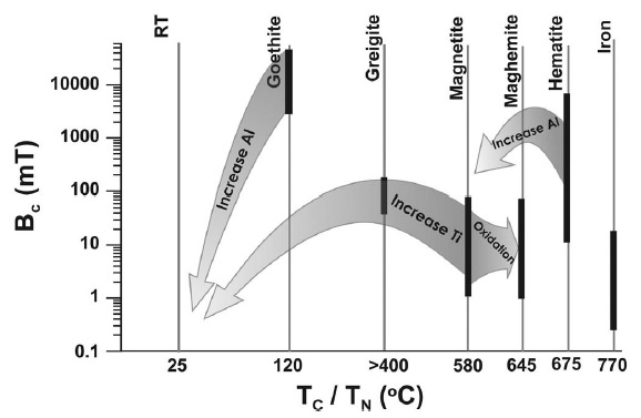
Figure 5 A schematic correlation of coercivity, Bc, with Curie temperature, Tc, and Neel temperature, TN, for different magnetic minerals. Arrows indicate the effects of isomorphous substitution and oxidation on the corresponding magnetic properties of these minerals. The thicker lines indicate coercivity ranges for different minerals. RT indicates room temperature. Figure taken from Liu et al. (2012).
By gradually lowering the temperature below Tc, the thermal energy overcomes the magnetic anisotropy until the remanent magnetization blocks in at the blocking temperature (Tb). With increasing grain size, Tb approaches Tc. Natural samples usually have a broad grain size distribution so that the maximum Tb is often equivalent to Tc (Liu et al., 2012). Through the substitution of iron with titanium, saturation magnetization Ms decreases and Tc decreases nearly linearly (Evans and Heller, 2003).
Magnetite is one of the most common ferromagnetic (s.l.) minerals found in natural samples. It appears totally opaque in microscope thin sections. Its high spontaneous magnetization (Ms) makes it the most magnetic naturally occurring mineral. Ti-magnetite is naturally formed in a variety of igneous rocks; as a result of weathering and erosion the minerals find their way into the natural cycle. Hematite is an iron oxide common in soils and sediments. Its spontaneous magnetization is about 200 times weaker than magnetite. It is, nevertheless, thermally more stable than magnetite due to its higher Tc. Below the Morin transition at −15ºC, hematite loses its magnetization (Evans and Heller, 2003). Maghemite occurs widely in soils and its chemical formula is simility to that of hematite, but with a different crystallographic structure. Maghemite is fully oxidized magnetite and has the same cubic structure. The spontaneous magnetization is slightly lower than that of magnetite. The Tc is often stated as around 645ºC, but Tc of maghemite is experimentally difficult to determine because maghemite is thermally metastable. At increased temperatures, between 200 and 900ºC, its crystallography irreversibly changes to hematite. This inversion temperature depends on impurities in the crystallographic lattice and grain sizes (Evans and Heller, 2003). Goethite is an iron oxyhydroxide with a hexagonal structure. Magnetic iron sulphides like Goethite are commonly found in reducing (anoxic) environments (estuarine mud), where organic matter is consumed by bacteria in the absence of oxygen (Rai, 2013). Zheng and Zhang (2008) observed Goethite in street dust and topsoil samples from Beijing. Its occurrence was evidenced in a peak around 280-300ºC in thermomagnetic curves that indicated the transformation from goethite to maghemite.
Iron sulfides such as pyrrhotite and greigite have become of great importance in studies of environmental pollution, because they act as “sinks” for toxic heavy metals (Dekkers and Schoonen, 1994; Snowball and Torii, 1999;). Pyrrhotite occurs naturally as an authigenic component in relatively old rocks, in present-day marine environments, in deep-sea cores, and in terrestrial sequences (Snowball and Torii, 1999). Greigite is commonly found in nature in ore deposits, lake sediments, and soils, or is formed in bacteria. Metallic iron, mixed with magnetite, has been found in indoor dust samples from apartments in the city center Zyrardow situated south-west of Warsaw, Poland (Górka-Kostrubiec and Szczepaniak-Wnuk, 2017). The metallic iron was mainly identified through its Tc of around 770ºC. Iron was also observed in Chinese street dust samples, but not in topsoil samples from the same locations (Zheng and Zhang, 2008). The absence of elemental iron in the topsoil samples was interpreted by the transformation of iron into iron-containing minerals by redox or other chemical reactions with organic matter. Muxworthy et al. (2002) combined magnetic measurements and Mössbauer spectroscopy on dust samples collected in Munich, Germany. Both methods identify a maghemite-like phase and an iron/maghemite phase, which they interpreted as an independent maghemite phase and a metallic iron phase with a maghemite shell. Maghemite was attributed to automobiles, whereas the metallic iron to electric street-trams, which closely pass by the sampling site.
The metallic iron content constitutes about 1% of urban atmospheric PM, of which 10-70% is made up of iron oxides and hydroxides (Muxworthy et al., 2002). Large amounts of this iron are attributed to mobile sources, such as vehicles. Moreover, iron impurities in fossil fuel convert during combustion to magnetic iron oxides, i.e. magnetite, maghemite, hematite, or a mixture, depending on the combustion conditions. The combustion of coal is one of the anthropogenic sources of magnetic fly ash. In an experiment, Liu et al. (2017) combusted iron-bearing coal at different temperatures and investigated its transformation behavior and the magnetic characteristics of the fly ash. During the combustion process, pyrite and siderite transform into iron oxides. They found that with increasing temperatures the relative content of magnetite and maghemite decreases, while hematite increases. In topsoil next to a road, Hoffmann et al. (1999) found that magnetite is the principal magnetic mineral for the enhancement of magnetic susceptibility.
This magnetite is believed to mainly arise from abrasion products from asphalt and from vehicle brake systems.
Kopcewicz and Kopcewicz (2001) investigated iron compounds of aerosols in Poland using Mössbauer spectroscopy. They found a significant amount of iron sulfides (FeS2, FeS, Fe1-xS) in winter, which they attributed to combustion of coal from house heating. Furthermore, they identified iron oxyhydroxides and iron oxides, mostly α-Fe2O3, originating from automobile exhaust.
4. Magnetic parameters
Magnetic parameters give insight into the domain state and grain size, the magnetic mineralogy, and the concentration of magnetic minerals in the sample. Detailed explanations of the physical background of magnetization and different domain states has previously been published (Thompson and Oldfield, 1986; Dunlop and Özdemir, 1997; Evans and Heller, 2003).
4.1. MAGNETIC SUSCEPTIBILITY
Magnetic susceptibility is one of the most commonly used mineral magnetic parameters. It is the ratio of induced magnetization (M, dipole moment per unit volume or J, dipole moment per unit mass) to the applied weak magnetic field (H) and expresses the capability of a material to be magnetized under the effect of an external magnetic field. Only for isotropic substances the induced magnetization is strictly parallel to the applied field, and the magnetic susceptibility is a scalar. In the general case of anisotropic media, like minerals and rocks, the induced magnetization is not parallel to the applied field, and the magnetization induced along the direction i is related to the magnetic field acting along the direction j by:
Ji = χijHj (mass specific) χ m3/kg
or
Mi = kij Hj (volume specific) k is dimensionless
Magnetic susceptibility mostly depends on the concentration and grain size of ferromagnetic (s.l.) as well as the contribution of para- and diamagnetic particles in a rock. For magnetite, magnetic susceptibility at low frequencies (klf or χlf) is remarkably constant over a wide range of grain sizes; it is, however, particularly sensitive to magnetite ultrafine magnetite particles, e.g., superparamagnetic (SP) particles in the 0.01-0.03 µm grain-size range. The frequency dependence can be used to detect these very small grains (Forster et al., 1994; Dearing et al., 1996). The frequency dependence of magnetic susceptibility (kfd or χlf), using magnetic susceptibility at low and high frequency (klf or χlf, and khf or χhf), respectively, is defined as kfd = ((klf − khf)/klf) × 100%. At a low frequency ω, corresponding to a period, 1/ω, larger than the relaxation time (1/ω > λ), SP grains contribute strongly to the susceptibility. Whereas the same grain becomes SD at high frequencies corresponding to a period smaller than the relaxation time (1/ω < λ). At a low frequency, SP grains equilibrate and can have higher susceptibilities than single domain (SD) grains. It is suggested that samples with kfd > 10% have dominating contribution of SP particles (Dearing et al., 1996). The frequency dependence of magnetic susceptibility reflects the concentration of SP grains, and particularly those close to the threshold SP-SD, that is 0.015-0.025 µm for magnetite (Maher, 1988). SD particles are extremely stable carriers of remanent magnetization with frequency‐independent magnetic susceptibilities. In contrast, SP particles just below the blocking volume of SD are unable to retain a stable remanence, but their susceptibilities are highly frequency dependent. The actual magnetic behavior of ultrafine magnetic particles, i.e., the observation of a SP or blocked state, largely depends on the value of measuring time (tm) of the specific experimental technique with respect to the relaxation time (t) (Wang et al., 2010). Figure 6 shows an example of frequency-dependent magnetic susceptibility at a college in Jalingo, Nigeria. Values of χFD > 10% indicate a large contribution of SP particles. The scattergram shows that the largest contribution to magnetic susceptibility is due to SP ferromagnetic grains <0.05 µm (Kanu et al., 2014).

Figure 6 A schematic χlf-χfd % scattering diagram showing samples from Jalingo College of Education, Nigeria (reproduced from Kanu et al., 2014, licensed under CC-BY-NC-ND 4.0, https://www.sciencedirect.com/science/article/pii/S0016716914700753).
Continuous thermomagnetic curves, which are magnetic susceptibility or saturation magnetization versus temperature (χ-T or Ms-T curves), in a saturation field of 1 T, are measured to determine the predominant magnetic minerals in the sample and their thermal stability (Goguitchaichvili et al., 2001). For the high-temperature curves, samples are usually heated to temperatures up to 700ºC and subsequently cooled to room temperature, while the magnetic susceptibility or magnetization is monitored. Commonly, the Curie temperature, which is typical for each magnetic mineral, is determined from the heating curve. The thermal stability is highest if heating and cooling curves overlap completely. The low-temperature thermomagnetic curves χ-T are measured while the sample is heated from temperatures as low as about −196ºC to room temperature. An example of low- and high-temperature thermomagnetic curves is shown in Figure 6 for four different materials (Sagnotti et al., 2009). In the low-temperature thermomagnetic curve an increase with maxima at −60ºC for the brake sample (Figure 7b) and at −30 to −50ºC for the other specimens was observed. In the high-temperature part of the thermomagnetic curves a Tc of ~580ºC was observed in the heating curve for all specimens, indicating magnetite as the main magnetic mineral.
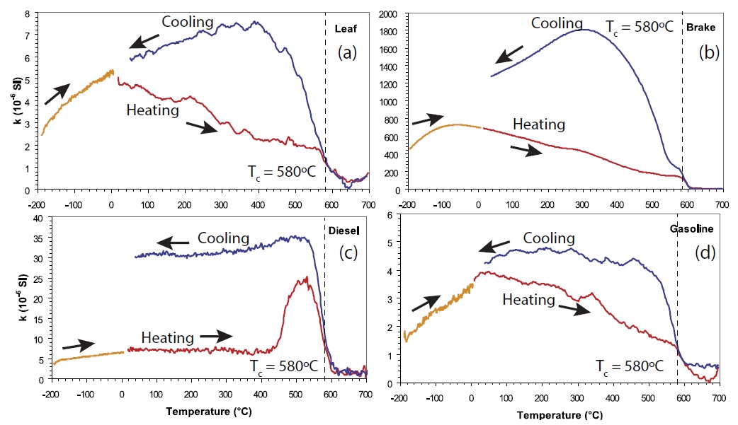
Figure 7 Thermomagnetic susceptibility curves for the four types of specimens, showing the changes in volume magnetic susceptibility during heating back to room temperature after cooling to liquid nitrogen temperature (orange) and during a heating (red)-cooling (blue) cycle from room temperature to ~700ºC. The high-temperature cycle was measured in an argon atmosphere (modified after Sagnotti et al., 2009).
4.2. MAGNETIC HYSTERESIS, DAY PLOT, AND FIRSTORDER REVERSAL CURVES
Magnetic hysteresis is a property of all ferromagnetic (s.l.) minerals, causing the magnetization of such a material to be strongly dependent on its magnetic history. The magnetization of a material is measured in dependence of an increasing and decreasing magnetic field. Parameters obtained from hysteresis loops are the saturation magnetization (Ms), remanent saturation magnetization (Mrs), and coercivity (Bc) (Figures 8a to 8c). Another approach to detect SP particles, besides the frequency dependence of magnetic susceptibility, is through measurements of hysteresis loops at very low temperatures. At low temperatures, SP particles behave like SD particles and can retain a remanence that is visible in the hysteresis loop (Radhakrishnamurty et al., 1971). However, these particles are not necessarily the same as those responsible for large χfd.

Figure 8 (a-c) Hysteresis curves. (d) Day plot. (e) First Order Reversal Curves (FORCs) (modified after Sagnotti et al., 2009).
The Day plot (Day et al., 1977; Dunlop, 2002a; 2002b) shows Mr/Mrs versus Bcr/Bc, with Bcr the remanence of coercivity obtained from the backfield curve measurement (application of an opposed incremental magnetic field). The Day plot, defined for magnetite only, indicates the grain size range of the magnetic minerals (Figure 8d).
First-order reversal-curve (FORC) diagrams are used to detect grain size distributions and can reveal signatures of SP particles (Pike et al., 1999). FORC diagrams make it possible to define the detailed coercivity distribution of the magnetic particles and their interaction field strengths. FORCs are a series of partial hysteresis loops made after the sample magnetization is saturated in a large positive applied field. To better visualize the produced set of loops, they are transformed into contour plots by calculating the second derivative of the measured magnetization, usually referred to as FORC diagrams (Figure 8e).
4.3. TYPES OF REMANENT MAGNETIZATION
Remanent magnetization is the magnetization that remains in a ferromagnetic (s.l.) mineral after removing a magnetic field. On the contrary, dia- and paramagnetic minerals cannot retain a remanent magnetization. Natural remanent magnetization (NRM) is obtained through natural processes, whereas other types of remanent magnetizations can be imparted in the laboratory in order to gain information about the ferromagnetic (s.l.) carriers of the samples.
Anhysteretic Remanent Magnetization (ARM) is the magnetization produced by the simultaneous employment of an alternating magnetic field (AF) and a direct current (DC) field. The magnitude of ARM depends on the applied AF and DC fields (Liu et al., 2012). Usual values of AF fields are 100 mT and DC fields are 50 µT.
All magnetic particles with coercivity lower than the maximum applied AF will remain aligned parallel with the direction of the bias field. The ARM intensity depends mostly on the concentration of fine SD particles. ARM is proportional to the DC bias field, and therefore, the anhysteretic susceptibility (χARM) is defined as the ratio of ARM over the bias magnetic field, (χARM = ARM/DC bias field; e.g., Liu et al., 2012). The χARM is strongly dependent on magnetic particle concentrations. Therefore, ARM can decrease with increasing concentration as shown on SD magnetite by Sugiura (1979).
In order to differentiate grain sizes of magnetite, Banerjee et al. (1981) suggested plotting the specific ARM (or χARM) versus low field χ. The magnitude of ARM given in a small steady field is sensitive to finer grain sizes, while χ is more sensitive to coarser grain sizes. In the sediment core samples of Banerjee et al. (1981) they found that small slopes in the ARM-χ plot indicate a paucity of fine grains. On the contrary, steep slopes show an increase of finer grains. King et al. (1982) constructed a simple phenomenological model based on magnetite grains with different sizes that were plotted in the χARM-χ-plot. This model enabled King et al. (1982) to detect changes, not only in grains sizes, but also in the amount of magnetite in natural samples, and is traditionally applied as “King-plot.”
Isothermal Remanent Magnetization (IRM) is the magnetization produced by the application of a pulse magnetic field at a constant temperature. The highest IRM value that may be obtained in a rock is defined as the saturation IRM (SIRM or Mrs). In nature, lightning may produce a high-intensity IRM, generally of low stability. The IRM (or SIRM) strength of a sample depends on the concentration of ferromagnetic (s.l.) particles. However, a field of 1 T will not saturate antiferromagnetic minerals like hematite and goethite (Liu et al., 2012).
The median destructive field (MDF) is the value at which half of the peak remanent magnetization is lost. It mostly depends on coercivity, and therefore on the composition of the magnetic grains.
4.4. S-RATIO AND OTHER RATIOS
The advantage of calculating ratios of magnetic parameters is that the dependence of these parameters may be eliminated. However, this assumption is only valid if the concentration of magnetic minerals is not too high, which may be influenced by grain interactions (Robinson, 1986).
The S-ratio is the ratio between the SIRM and the backfield IRM produced by applying a pulse field (typically of 0.1 T or 0.3 T) in the opposite direction of the previously applied field used to produce the SIRM: S−0.1 T = −IRM−0.1T/SIRM or S−0.3 T = −IRM−0.3T/SIRM (Liu et al., 2012). It mostly depends on the composition of the magnetic grains. S−0.3 T is used mostly to estimate the relative amount of low- and high-coercivity minerals, or between ferrimagnetic and (canted) antiferromagnetic minerals (Robinson, 1986). S−0.1 T may provide an estimate of the relative amount of low-coercivity ferromagnetic grains (e.g., multidomain magnetite). Hence, an S-ratio that converges to unity indicates that ferrimagnetic minerals are dominant (Liu et al., 2012); in other words, it discriminates between ferrimagnetic and (canted) antiferromagnetic minerals.
The hard IRM (HIRM) is defined as (SIRM + IRM−0.1T)/2 or (SIRM + IRM−0.3T)/2. It depends on the concentration of minerals with coercivity higher than the applied backfield.
For weak magnetic mineral concentrations (i.e., in absence of significant magnetic interaction), concentration-dependent rock magnetic parameters vary linearly, at least in first approximation, with the abundance of magnetic particles in a specimen. The ratio of two concentration-dependent rock magnetic parameters can be used to infer trends of variation in the grain size and magnetic domain state in a rock sequence. For example, ARM/k is used to estimate the variation in the grain size and magnetic domain state of magnetite particles. The ARM/χ ratio is inversely related to the size of magnetite grains.
SIRM/k or SIRM/χ, analogously to ARM/k or ARM/χ, is used to estimate variation in the grain size of magnetite particles (e.g., Rai, 2013). With respect to ARM/k, SIRM/k is more sensitive to changes in the proportion of large grains (>10 mm). Both parameters vary inversely with the magnetic grain size; however, SIRM/k varies over a wider range than ARM/k (Thompson and Oldfield, 1986). Additionally, SIRM/χ has been used as an indicator for SD greigite grains in sedimentary environments (Liu et al., 2012).
SIRM/ARM is also a parameter used to estimate grain-size changes in populations of magnetite grains. SIRM/ARM increases as the magnetite grain size increases. This ratio is, however, less sensitive than ARM/k and SIRM/k. An advantage of SIRM/ARM is that it depends only on remanence and is therefore unaffected by SP grains. The ratio χARM/SIRM is a grain-size indicator (Peters and Dekkers, 2003; Rai, 2013), while Zhou et al (2015) identified this ratio as the most powerful parameter in discriminating different pollution sources.
The ratio of saturation remanent magnetization (Mrs) to susceptibility, Mrs/χ is useful to assess the magnetic mineralogy, e.g., high ratios point to pyrrhotite, intermediate to greigite or maghemite, and low values may indicate Ti-magnetite (Peters and Dekkers, 2003).
5. Non-magnetic measurements of pollution agents
In general, magnetic measurements are often accompanied by chemical analyses in order to identify the heavy-metal concentrations in the samples. Several studies use X-ray fluorescence (XRF) spectrometry to determine the total heavy metal content (e.g., Yang et al., 2007; Aguilar Reyes et al., 2011; Wang et al., 2012). A mineralogical characterization can be performed using X-ray powder diffraction (XRD; Bourliva et al., 2017). X-ray energy dispersive spectrometry (EDX) is applied to identify the elemental composition (Yang et al., 2007; Zhang et al., 2012; Bourliva et al., 2017).
Several new techniques based on X-ray photon absorption produced at synchrotron radiation facilities have been applied to investigate magnetic properties at the atomic scale (Liu et al., 2012). Their advantage is that they are independent of the physical state of a sample, as opposed to, for example, XRD analysis. One of these techniques, X-ray absorption spectroscopy, helps investigating the oxidation state, bonding, and arrangement of neighbor atoms. It can further be used as a fingerprint to compare unknown samples to standards. X-ray magnetic circular dichroïsm (XMCD) and scanning transmission X-ray microscopy (STXM) are two more methods to investigate magnetic properties. The total amount of heavy metals in a bulk soil sample, and in the magnetic and non-magnetic fractions, can be determined by Inductively Coupled Plasma Mass Spectrometry (ICP-MS).
An important factor in the estimation of health risks is the bioavailablity, because not 100% of contaminants are bioavailable, meaning, available for the human body for assimilation (Bourliva et al., 2017). Bourliva et al. (2017) determined the vitro oral bioaccesibility of Pb and Zn using the unified bioaccessibility method. This approach simulates leaching of a solid matrix in the human gastro-intestinal tract. Aguilar Reyes et al. (2011) determined the bioavailablity of heavy metals by first extracting heavy metals using diethylenetriamine penta-acetate, and subsequently measurements with a spectrometer of atomic absorption. Scanning electron microscope analyses help identify associations between magnetic minerals such as magnetite and heavy metals (Aguilar Reyes et al., 2013) or the overall size distribution and morphology of particles (Urbat et al., 2004; Jordanova et al., 2008; Lu et al., 2011; Chaparro et al., 2013; Castanheiro et al., 2016; Castañeda Miranda et al., 2016; Bourliva et al., 2017).
In the case of soils, various measurements can be performed in order to characterize the physico-chemical properties of soils. For example, Bourliva et al. (2017) determined the pH of soils, the soil organic matter by the loss-of-ignition procedure, the soil organic carbon content by non-dispersive infrared method (NDIR), and the carbon exchange capacity, among others.
A valuable method to characterize the iron content is the Mössbauer spectroscopy. This type of measurement allows not only determination of the content of the isotope in the sample but also identification of the chemical compound in which the isotope appears (Kopcewicz and Kopcewicz, 1978; Kopcewicz and Kopcewicz, 2001). Mössbauer spectroscopy at different temperatures is used to estimate the size of the iron-containing particles (Kopcewicz and Kopcewicz, 1978). Muxworthy et al. (2002) combined thermomagnetic measurements with Mössbauer spectroscopy to identify the high-temperature magnetic phase as iron.
6. Magnetic monitoring of anthropogenic pollution in urban areas
6.1. DIRECT MONITORING AND FORECASTING OF ANTHROPOGENIC POLLUTANTS
Active monitoring of PM with air quality monitoring stations or in air filters allows obtaining localized time series of particle concentrations. Active collection onto air filters allows the differentiation of various size classes (e.g., Lehndorff et al., 2006). For example, Heo et al. (2017) analyzed hourly PM10 mass concentration data for 16 years from Seoul (Korea). This direct measurement allowed them to observe a stagnation of the decline of mass concentration with the final goal to take action to improve air quality. Revuelta et al. (2014) carried out a combined magnetic-chemical study of 15 daily PM (PM10, PM2.5 and PM1) aerosol samples in Barcelona, Spain. They distinguished crustal sources of North Africa from other sources of PM1.
In order to react to changes in PM levels and to warn the population of unfavorable conditions, policy makers need reliable forecasting models of daily PM concentrations. Stadlober et al. (2012) suggested a multiple linear regression and generalized linear models for the sites of Graz, Austria and Brno, Czech Republic as suitable monitoring tools and as a base for decision makers. Perez and Reyes (2006) applied an integrated artificial neural network model to predict the maxima of the 24 hour average of PM10 in Santiago, Chile. Their model takes into account the spatial pattern of PM10 distribution during the evening of a given day in order to forecast the concentration at the same stations the next day.
Recently, the differential absorption lidar (DIAL) technique has been applied in a mobile system to detect the total flux of certain pollutants such as SO2 and NO2 (Zhao et al., 2017). Of special interest for China is the monitoring of atomic mercury (Hg), which is considered a particularly hazardous heavy-metal pollutant. With the mobile DIAL system, Hg can be monitored in ranges of typically a few km. As part of the mobile system a remote laser-induced break-down spectroscopy (LIBS) system also allows the detection of the elemental composition in soils.
In the last few years, atmospheric concentrations of PM10 have been measured as well with satellite remote sensing systems. This space-based monitoring, based on Aerosol Optical Depth (AOD) measurements, e.g., from the MODIS sensor onboard the Aqua Satellite, is a quantitative measure of the amount of the depletion that a beam of solar radiation undergoes as it passes through the atmosphere. Michaelides et al. (2017) analyzed satellite data with a resolution of 10 × 10 km.
6.2. BIOMAGNETIC MONITORING
Airborne pollution exposure data obtained from networks of monitoring stations frequently have a low spatial resolution and are therefore not able to capture small-scale variations in PM concentrations and particle size. Monitoring stations are often several kilometers apart, which impedes identifying and quantifying causal links between the degree of exposure to PM and the likelihood of adverse health impacts within a population. Furthermore, conventional monitoring stations are generally located far from residential areas and often situated above 3 m height (Mitchell et al., 2010). Therefore, biomagnetic monitoring of PM has the potential to provide spatial and temporal high-resolution data of polluted areas (Matzka and Maher, 1999; Mitchell et al., 2010; Hofman et al., 2017). Furthermore, it is more economic and faster than many geochemical methods. The ability to capture fly ash and magnetic particles depends very much on the type of surface, e.g. tree trunk bark is about two orders as effective as certain leaves (Evans and Heller, 2003), while the receptor material needs to be insignificantly magnetic.
6.2.1. PLANTS, MOSSES, AND LICHENS
Mitchell et al. (2010) investigated PM10 deposition on birch and lime tree leaves, both on initially “clean” (glasshouse grown) specimens and on roadside trees and found that PM gradually accumulated on the surfaces of deciduous tree leaves until a dynamic equilibrium between particle deposition and particle loss is reached. For birch and lime trees, the time required for equilibrium to be reached is of the order of 6 days. When dynamic equilibrium has been reached, leaf SIRMs can act as a quantitative measure for ambient PM10 concentrations. The main processes involved in reaching dynamic equilibrium are dry deposition and particle re-suspension, both driven by air turbulence.
Some authors found conifers more reliable than broadleaf trees due to higher deposition velocities for fine to ultrafine particles and due to higher capture efficiency (e.g., Beckett et al., 2000). Furthermore, a contrasting relationship has been reported between leaf SIRM and exposure time for waxy evergreen and deciduous leaves. For Pinus nigra, for example, Lehndorff et al. (2006) observed an increase in needle SIRM during the first 20 months, with an equilibrium reached after approximately 26 months of exposure. Such long equilibration times suggest that the leaf SIRM is dominated by incremental incorporation of magnetic particles within the cuticular structure.
Rai et al. (2016) tested Lantana camara as a biomonitor, which is the most dominant weed in Aizwal, Mizoram, India. Samples collected in rural areas have lower values of magnetic susceptibility and remanent magnetization compared to samples from urban areas. Lantana camara proves to be a suitable biomonitor for PM (Rai et al., 2016).
Barima et al. (2014) investigated the potential of leaves from four different herbaceous and tree species as a bioindicator of urban PM pollution. The four species were selected based on their distribution in different land use classes, their convenience to harvest, and the width of their leaves for easy scanning. The species were Amaranthus spinosus, Eleusine indica, Panicum maximum, and Ficus benjamina, all plants that are home to the tropical urban environment of Abidjan, Ivory Coast. Barima et al. (2014) showed that the SIRM is at least four times higher in the vicinity of main roads and industrial areas than in parks and residential areas. Distances of 0-5 m seem to be most affected by PM pollution. The slightly hairy leaves of Amaranthus spinosus and the waxy leaves of Ficus benjamina had largest SIRM values.
Giordano et al. (2013) found that the accumulation of urban PM from Naples, Italy was highest in moss (Hypnum cupressiforme), followed by lichen (Pseudevernia furfuracea), and finally cellulose filters, with the lowest accumulation capacity. They further found that the elemental uptake increased during rainy periods. Especially oven-dried moss preserved a high elemental accumulation capability. Jordanova et al. (2010) performed a detailed study on different vegetation samples (lichens, mosses, poplar leaves, dandelion, and needles) for several highly polluted and clean sites in Bulgaria. They conclude that lichens and mosses have higher accumulation capacities and therefore they can be the best biogenic dust collectors.
6.2.2. SOIL CONTAMINATION
Boyko et al. (2004) tested the repeatability of magnetic susceptibility mapping in two field campaigns on 129 sites in North and West Austria on a regular grid of 10 × 10 km and on a high-resolution grid of 2 × 2 km in the polluted Steyreggerwald near the town of Linz. The measurements obtained with a Bartington Instruments MS2D handle were compared with magnetic susceptibilities of soil reference material taken at the measured sites. The Bartington handle measures susceptibilities in the top 6-8 cm, whereas for the reference material the upper 3.5 cm of the topsoil were sampled. Boyko et al. (2004) found significant correlation between magnetic susceptibilities from the readings in the field with the ones of the reference material. Especially for the high-resolution grid, the 33 topsoil measurements reveal high correlation (R2 = 0.98; Figure 9). Factors that affect the repeatability of the field measurements are, for example, inhomogeneities within the measured place, positional precision, different equipment sets, plant cover, and anthropogenic activity.

Figure 9 Results of the high-resolution screening of Linz area. Ratio of volume magnetic susceptibility of the soil reference material versus susceptibility measured in field (Boyko et al. 2004).
Soils contaminated by mining and processing industry are often recultivated to restore the natural environment (Jordanova et al., 2017). Jordanova et al. (2017) applied magnetic methods to determine the degree of soil restoration close to a metallurgical copper-processing plant in Bulgaria. They found an enhanced amount of magnetite in the uppermost levels of the Technosol, which may have formed through the reduction of hematite that was initially present in the dump material. Magnetic grain size proxies (ARM/IRM100mT, χfd%) identify magnetic grains larger than SP grains, suggesting that the enhanced magnetic signal partly originates from fly ash additions to the soil. Fly ash, commonly in the form of alkaline ash from industrial processes, is often applied in soils for restoration purposes as a liming agent (Jordanova et al., 2017). However, χ in the uppermost level shows a linear positive trend with the age of the forest stand, indicating that the magnetic enhancement may be linked to pedogenic processes. Furthermore, depth variations of the magnetic parameters along the soil profiles suggest that with time after recultivation, magnetic particles from pedogenic processes and/or from fly ash spread progressively deeper, reaching about 15 cm in the 25-year-old silver-birch forest.
Li et al. (2017) combined magnetic methods with XRF and other non-magnetic methods to investigate the fate of heavy metals in different types of soil horizons. The heavy-metal contents may differ in particular soil horizons because soils are governed by their proper physicochemical properties such as pH, soil moisture, and amount of organic matter and clay minerals. They found a clear difference between the red clay horizon and the upper and lower yellow silt horizons; the χlf signal was stronger in the clay horizon due to a higher amount of ferromagnetic (s.l.) minerals in the iron-bearing clays and mafic silicates, consistent with higher weathering and pedogenic processes compared to the silt layers (Li et al., 2017). The clay layer also showed values of χfd% > 6%, that were higher than those in the silt layer, indicating larger amounts of SP grains. The trend in the clay layer with higher magnetic susceptibility values correlates with mean concentrations of heavy metals 1.5 times higher than in the silicate layer.
6.2.3. STREET DUST
Cortés et al. (2015) calculated color indices for dust collected on urban streets. They used the RGB system and grouped each color using the Munsell tables (Munsell Color, 2000). Results were compared to XRF measurements to identify the elements contained in the dust samples. The study showed that Rb and V are present in largest concentrations in dark red dusts, while Ni, Cu, Zn, and Pb are mainly present in gray dusts. In general, ash produces gray colors, whereas red and brown colors often stem from local soils. However, for each city or sampling area, colors should be determined beforehand in a reference study (Cortés et al., 2015). Xie et al. (2000) investigated the organic matter content, e.g., PAH, of street dust in Liverpool, UK. Their main goal was to determine if magnetic measurements correlate with organic matter content. In order to quantify the organic matter content, weighed samples of dust were oven dried at 105ºC overnight, reweighed and then ignited in a muffle-furnace. The loss-on-ignition method is a common technique to estimate organic matter content in soil samples. Ignition at 375ºC for 16 hours worked best to remove organic matter without structural water loss from inorganic components. The loss of inorganic carbon compounds is reported to start at temperatures >400ºC (e.g., Xie et al., 2000). The amount of organic compounds was determined to be 4 ± 1.3%. Magnetic measurements indicate that the main magnetic grain sizes are MD grains, with smaller amounts of SP and SD grains. Furthermore, Xie et al. (2000) found the strongest correlation between organic matter content and χfd (R = 0.607), suggesting that magnetic methods can be useful proxy methods for organic matter in street dust.
6.2.4. CONTAMINATION OF URBAN RIVERS, HARBORS, LAKES, AND SEAS
Zhang et al. (2011) focused on the discrimination between contributions of different pollution sources in urban river sediments from Loudi City, Hunan Province, China. Furthermore, they aimed to establish a relationship between magnetic parameters and heavy metal contamination, obtained from chemical, microscopic, and statistical methods. The magnetic investigation revealed that PSD and MD magnetite occur as dominant ferromagnetic phases, with small amounts of SP particles. The SP magnetite particles likely came from pedogenic processes in the subtropical region. Some heavy metals found in the sediment (Be, Cs, Rb, Nd, Co, Ni, Ba) do not correlate with the magnetic parameters. Their main sources were probably pedogenic processes in the catchment region upstream. On the contrary, Fe, V, Cr, Mo, Zn, Pb, Cd, and Cu showed a significant correlation with Ms, χ, χARM, and, especially, with SIRM, suggesting that these metals and their related magnetic particles stem from anthropogenic sources from the urban zone. Furthermore, SIRM does not include the contribution of pedogenic SP particles, making it the optimum proxy parameter for the detection of heavy metals in river sediments. Knab et al. (2006) investigated the influence of complex geological settings, with magnetically strong rock formations, on the magnetic signal of river sediments from the river Moldau, Czech Republic. They used magnetic susceptibility, which has been shown to reflect industrial input into river sediment, to distinguish between anthropogenic and natural contribution in river sediments (Knab et al., 2006). By comparing susceptibility measurements from outcropping rocks, soils close by the river, and river sediments, they found that the geological background value should be considered locally as a magnetic source of primary significance. Nevertheless, the anthropogenic contribution could be clearly observed in areas of minor lithogenic contribution (Knab et al., 2006). In another approach, Frančišković-Bilinski et al. (2014) measured χ and IRM from predominantly unpolluted rivers from Croatian and Slovenian flysch areas and compared the results to several rivers and a lake from the Celje old metallurgic industrial area (Slovenia). Sediments from the unpolluted flysch rivers had extremely low χ and IRM values, with mass susceptibility between 0.6 and 5.1 × 10⁻⁷ m3/kg and IRM between 0.7 and 7.9 A/m. On the contrary, in the industrial area χ and IRM were much higher with χ between 1.3 and 38.3 × 10⁻⁷ m3/kg and IRM between 0.9 to 100.4 A/m. The highest χ values were found in an area where significant amounts of heavy metals were reported in earlier studies. Sediments of the industrial area have mostly diamagnetic quartz as a major lithogenic mineral, with small amounts of carbonate, while in sediments of the flysch (karstic) rivers, carbonate minerals dominate.
6.3. METEOROLOGICAL, CLIMATIC, TEMPORAL, AND SOURCE-RELATED EFFECTS
Concentrations of magnetic particles are governed by exposure time, source distance, source strength, and sampling height, as well as number and intensity of rainfall events, and wind velocity and direction (e.g., Hofman et al., 2017). Rainfall events lower both ambient PM10 concentrations and magnetic parameters of leaves, but contrasts have also been reported for different plant species (Mitchell et al., 2010). For deciduous leaves, Mitchell et al. (2010) reported a decrease in magnetic strength of leaves due to rainfall effects and suggested that rain-induced wash-off of magnetic particles from tree leaves is likely to vary according to species and leaf characteristics, in addition to rain intensity, canopy position, and degree of shelter. For pine needles, Urbat et al. (2004) demonstrated that rainfall removes only a small portion of the captured PM, as particles are trapped in the surface wax layer and stomatal pores. For another evergreen species, Quercus ilex, Szönyi et al. (2008) reported no clear indication that rain systematically decreased the intensity of leaf magnetic properties. However, Zhang et al. (2006) observed that the magnetization for pine trees (Pinus pumila) was lower at a later sampling event compared to an earlier sampling event, which they explained by a heavy rain event prior to the later sampling. At least half of the magnetic susceptibility signal was removed by the heavy rain. However, the magnetic signal was still significant and had a sample-distance dependence, suggesting that rain cannot completely remove the accumulated PM. Kardel et al. (2011) showed a limited effect of rain-induced wash-off and a strong correlation with accumulated PM10 during the growing season, suggesting some time-dependent incorporation of magnetic particulates in the epicuticular wax layer. Xu et al. 2017 developed artificial rainfall experiments in order to investigate the effects of rainfall on PM wash-off mass. They used four broadleaf species, one of which was evergreen and the other deciduous. Not only rainfall duration but also intensity has an effect on PM wash-off. In addition, an exponential decay was observed between cumulative wash-off rates and rain amount.
Besides meteorological factors, climatic factors that act on larger time and spatial scales also affect the accumulation of pollutants on surfaces (Rodríguez-Germade et al., 2014). By comparing data from cities with different climatic regimes, e.g., subtropical monsoon, continental, oceanic and Mediterranean climates, Rodríguez-Germade et al. (2014) found that atmospheric humidity plays an important role in the accumulation of particles on leaves. Less humid climates, as well as low soil water availability, causes the leaves’ stomata to open, which increases the water loss by transpiration (Barceló et al., 2001; Rodríguez-Germade et al., 2014;). These effects enhance the leaves’ capacity to incorporate particles in their surface tissue. Besides the incorporation of particles, the lithic component of urban dust of the accumulated particles depends on atmospheric humidity. Rodríguez-Germade et al. (2014) noticed that the lithic component is stronger in arid regions where the relative humidity is low. Furthermore, they compared the correlation between different metal concentrations and magnetic susceptibility, and found lower correlation in cities with lower moisture.
In general, concentration of PM decreases as wind speed increases, although sometimes an increase in concentration was observed at highest wind speeds (Jones et al., 2010). A small portion of coarse PM was a result of wind-induced resuspension at higher wind speeds. Jones et al. (2010) found a relationship between the mean concentration (X) and the wind speed (U) for different metrics of PM and NOx, as laid out in the equation
where a1, a2, a3 are constants associated with emission of material from large-area sources, discrete local sources, and marine sources, and which can be determined for each metric and location; c and cʹ are constants that were chosen by iteration. For particulate nitrate, the reduction of concentration happens much faster, and the equation needs to be adapted.
Several studies have dealt with distance to source distribution of PM. For example, Maher et al. (2008) investigated tree leaves from roadside trees and found higher and strongly correlated lead, iron, and remanence values closer to roads. Values and correlations were also higher on road-proximal than road-distal leaves. Higher amounts of pollutants were found on tree leaves next to uphill than to downhill road lanes. Concerning the vertical distribution, Maher et al. (2008) found highest pollution with lead and iron at about 0.3 m and at 1.5-2 m height. Considering that common monitoring station collectors are placed at heights of 3 m, it can be supposed that they underestimate pollution concentrations.
6.4. ANTHROPOGENIC VERSUS NATURAL POLLUTANTS
In order to distinguish anthropogenic pollution from natural sources in terms of magnetic minerals, heavy metals, or organic compounds present in soils and dusts, several approaches have been suggested. To assess the contamination levels of heavy metals in soils, Müller (1986) introduced the geoaccumulation index, Igeo, in which the current and pre-industrial concentrations of elements are compared.
where Cn is the current concentration of elements in the environment, and Bn is the geochemical background value in soil. Müller (1969) divided the Igeo values in a scale ranging from Igeo ≤ 0 (uncontaminated) to Igeo ≥ 5 (extremely contaminated). The “enrichment factor,” the ratio of element concentration relative to crustal values, is used to distinguish between natural and anthropogenic contributions to heavy metal contamination in fly ashes. The highest enrichment factor was reported for Cd with a value of 2400, while Pb is in general lower with a value of 740 (Wadge et al., 1986). These authors also found an inverse relation between particle size and the enrichment factor. Another factor to quantify pollution is the contamination factor, CF (Hakanson, 1980). It is the ratio between a single heavy-metal concentration and its background or preindustrial value. CF < 1 indicates low contamination; 1 ≤ CF < 3 is a moderate contamination; 3 ≤ CF < 6 is considerable contamination; and CF ≥ 6 is very high contamination.
The pollution load index (PLI) of Tomlinson et al. (1980) is
where CFn is the contamination factor for the concentration of each heavy metal. The PLI can be used to compare pollution within different sites.
Spassov et al. (2004) developed a method for distinguishing and quantifying anthropogenic from natural pollution based on demagnetization curves of anhysteretic remanent magnetization (ARM). They calculated coercivity distributions from the demagnetization curves of ARM and modelled the components using a linear combination of specific functions. These functions represent the contributions of different sources of magnetic minerals. As a result, they suggested that the PM10 magnetic carriers can be divided in a high-coercivity component originating from exhaust emissions and a low-coercivity component that is derived from natural dust and traffic related pollution.
Magiera et al. (2006) investigated indications to discriminate between lithogenic and anthropogenic influences on magnetic susceptibility (χ) in top soils. From horizontal and vertical distributions of χ measured in topsoil cores, they found, among others, the following indicators of anthropogenic contributions: (1) susceptibility anomalies were observed close to industrial or urban sources of pollution, (2) the strongest enhancement of χ was found within the uppermost 8 cm, and (3) the enhancement of χ is accompanied by increased heavy metal content. On the contrary, they suggest the following indicators for a lithogenic origin of enhanced topsoil: (1) the anomalies are found in areas far from industrial or urban centers, (2) the enhancement of χ increases gradually with depth, and (3) heavy-metal content is generally low and not correlated to χ. The last point is related to the fact that the bedrock determines a large part of the soil type and its properties.
6.5. DISTINCTION BETWEEN DIFFERENT (ANTHROPOGENIC) SOURCES OF POLLUTION
Shu et al. (2001) showed that the combined magnetic and geochemical analysis in urban and industrial environments can jointly support the classification of different sources. Dust samples were collected at eleven locations across Shanghai, China. Magnetic susceptibility at low frequencies (χlf) and saturation isothermal remanent magnetization (SIRM) values are largest at sites with highest concentrations of Fe, Mn, Ni, V, and Zn. This correlation confirms that ferrous particles and magnetic spherules in emissions from heavy industry and coal-fired power plants are the main causes of high ferrimagnetic concentrations. Furthermore, magnetic measurements indicate that magnetite MD and PSD grains are largely produced in fossil-fuel combustions.
Zhang et al. (2012) determined the major sources of anthropogenic pollution in the city of Loudi, China through the spatial distribution of magnetic parameters such as magnetic susceptibility. They found that magnetic minerals that incorporate heavy metals mainly stem from an Fe-smelting plant, followed by traffic as the second largest source. Particles are distributed following the main wind direction.
Bivariate plots, or biplots, combining different magnetic parameters can be a powerful tool to discriminate between different anthropogenic sources. Lecoanet et al. (2003) examined which combination of magnetic parameters is most suitable to characterize soil samples. They found a good correlation between SIRM and χ with R2 = 0.83. Interestingly, the lowest SIRM and χ values were measured in roadside soil samples, and not in the natural soil background sites. Lecoanet et al. (2003) explain this observation on the one hand with a high paramagnetic content in the road side samples and, on the other hand with post-depositional weathering and/or formation of magnetic phases by pedogenic processes in the natural soil samples (Lecoanet et al., 2003). Also, Zhou et al. (2015) showed that bivariate plots of different magnetic parameters are efficient to discriminate between different sources of contamination. They found a strong correlation between χARM/SIRM and χARM/χ with clearly separated patches of soils from near a cement plant, near a coal plant, and from the roadside. Furthermore, the ratio χARM/ SIRM is sensitive to different grain sizes as well as to high- or low-coercivity minerals, e.g., hematite and magnetite/maghemite, respectively (Zhou et al., 2015). By making use of this ratio, Zhou et al. (2015) identified predominantly ferrimagnetic minerals (magnetite or maghemite) in soil samples from roadsides and near the power plant, and hematite from samples near the cement plant.
6.6. CORRELATIONS BETWEEN HEAVY METALS, MAGNETIC PARAMETERS, HEALTH-RELATED FACTORS, AND ORGANIC MATTER
Wang et al. (2012) investigated the magnetic properties and elemental concentrations of street-dust samples from four different districts. The highest concentrations of magnetic minerals, derived from the concentration depend parameters χlf, SIRM, “soft” IRM, HIRM and χ ARM, and heavy metals were found in the two industrial districts. A generally highly significant positive correlation between magnetic concentrations and those of As, Cu, Mn, Ni, Pb, and Zn corroborate that a large part of the heavy metals within the four districts is linked to particulate emissions from combustion processes. Through the combination of magnetic and element concentrations, distinct sources of heavy metals could be identified in the two industrial districts. The differences were on the one hand contrasting ferrimagnetic grain sizes, observed in the χfd%-SIRM plot, and, on the other hand, different ferrimagnetic-antiferromagnetic fractions, detected in the S-300-χlf plot.
Xie et al. (2000) investigated the organic content in street dust in Liverpool (UK) and found that it had the strongest correlation with χfd (R = 0.607). Therefore, the authors suggested that certain magnetic measurements may be suitable as proxies for organic content matter in street dust. However, Shilton et al. (2005) argued that data should be separated into site-specific correlations. They took street dust samples from three different roads with very different traffic patterns. When comparing the correlations χfd% and χARM/SIRM with the organic content for the three roads, differences were obvious. While χfd% seemed to be more consistent within all three roads, χ ARM/ SIRM exhibits completely different trends. Therefore, Shilton et al. (2005) concluded that there are significant correlations between organic matter in urban street dust and magnetic parameters, but the correlations can be very different, even within the same area.
Magnetic susceptibility of respirable pollutant particles has been shown to have a strong correlation to heavy metals such as Pb, Zn, Cd, and As and, furthermore, to their mutagenic potency, i.e., their ability to cause mutations in the genome (Morris et al., 1995; Ďurža, 1999; Petrovský et al., 2001; Shu et al., 2001; Morales et al. 2016). Morris et al. (1995) first indicated that there is a direct association between magnetic susceptibility and mutagenic potency of inhalable PM (content of PAH). They investigated 62 air filter extracts and found a high correlation between mutagenicity and magnetic susceptibility (Figure 10). The linear regression shows a correlation factor of R = 0.80. This indicates that χ may be used as an indicator for mutagenetic activity of respirable PM.

Figure 10 Mutagenicity (expressed as revertants, which is a mutant gene, individual, or strain that regains a former capability by undergoing further mutation per m3 of air) of polycyclic aromatic compounds and magnetic susceptibility (10-6 cgs per m3 of air) (Modified after Morris et al., 1995).
7. Discussion and critique
7.1. INTERNATIONALLY ACCEPTED THRESHOLD VALUES FOR POLLUTANT AGENTS
Research efforts have not yet found evidence for a safe level of PM exposure, below which negative effects for health do not occur. However, in the air quality guidelines (AQG) from WHO (2006) a maximum level of PM10 of 20 µg/cm3 as an annual mean was suggested. In 2010 only 9 of 34 member states were below this level. Recent estimates for PM2.5 were published as part of the Global Burden of Disease, Injuries, and Risk Factors Project. The threshold values of the AQG for PM2.5 are 10 µg/ m3 for an annual average and 25 µg/m3 for 24 hours, and for PM10 it is 20 µg/m3 for an annual average and 50 µg/m3 for 24 hours. Nevertheless, air pollution may be higher in areas with power plants, heavy traffic, and other sources. Different measures are required to be applied to protect the population in these areas (WHO, 2006). The critical period of exposure is most probably one year, e.g., exposure to PM2.5 reduces life expectancy by about 8.6 months on average. Health improvements can be expected to start almost immediately after reduction of air pollution (WHO, 2013).
It has to be noted that the AQG are recommendations and not binding standards. Air quality standards are meant to be defined by each country to protect their population, according to the WHO. These standards may vary according to the solutions applied for reducing air pollution based economic, political, and social factors, among others. Therefore, the WHO explicitly acknowledges that governments adopt their own standards depending on their country-specific circumstances (WHO, 2006). However, this non-binding AQG may avoid commitment of certain countries to reduce contamination. At least, a common upper level of contamination should be binding for all countries, such as one of the interim targets suggested by the WHO (WHO, 2006). These interim targets serve as milestones in reaching the AQG. Finally, ultrafine particles show high evidence of potential negative effects on health, but are not included in the AQG. There is still a lack of studies to be able to define common standards for these particles.
In the last few decades, the number of megacities-urban agglomerations with a population larger than 10 million people-have been growing (Baklanov et al., 2016). Most of the megacities are located in developing countries that do not have the necessary financial resources, air quality management plans, or political stability to counter heavy air pollution (Baklanov et al., 2016). Air pollution problems in megacities are influenced by topography, demography, meteorology, mobility and transportation patterns, fuel quality and usage, level and rate of industrialization, and socioeconomic development (Baklanov et al., 2016). Therefore, air quality standards need to consider the specific factors that produce and influence air pollution. Air pollution mitigation strategies should include the use of clean technologies and policy measures (Baklanov et al., 2016). However, there are still large socioeconomic and political barriers to the transition to new eco-friendly technologies (Baklanov et al., 2016).
Soil pollution by heavy metals has been a worldwide concern, and countries have developed laws and regulations to control them, e.g., the US, Mexico, Nigeria (US EPA, 1996; SEMARNAT, 2007; Wuana and Okieimen, 2011, respectively). However, there is no consensus on the permissible heavy metal concentrations, and much less on the amount of heavy metals per type surface. One of the most commonly used methods to determine the concentration of heavy metals in soil is the total element analysis (USEPA method 3050, Wuana and Okieimen, 2011). In general, the level of heavy-metal contamination is expressed as mg metal/kg soil. However, the total element analysis does not take into account moisture content, and may therefore alter the concentration by including soil water (Wuana & Okieimen, 2011).
7.2. DISCRIMINATION BETWEEN NATURAL AND ANTHROPOGENIC POLLUTION
The magnetic trace is composed of a natural and an anthropogenic contribution. Therefore, one of the main challenges is to discriminate between the two signals. Areas that are most magnetic are not necessarily the most contaminated-the amount of ferromagnetic (s.l.) minerals depends on lithological and pedological characteristics of the soil. A straightforward way to identify anthropogenic pollution is by comparing top- and subsoil samples (Hanesch et al., 2007). Contaminants accumulate, in general, in the uppermost centimeters of the soil (0-20 cm). Therefore, a higher magnetic value in the uppermost layer with respect to the subsoil indicates contamination. More specifically, a negative difference between the magnetic parameter of top- and subsoil is attributed to a highly magnetic bedrock (e.g., ore bodies), while a high positive difference is considered an anthropogenic anomaly (Hanesch and Scholger, 2002).
Additionally, statistical methods, such as the median absolute deviation methods, the boxplot method, the population modeling method, and the quantification of anomalous values by the Geoaccumulation Index identify anomalies of magnetic values that may be attributed to contamination (Hanesch et al., 2007). It is of major importance to bear in mind background values, because high magnetic values can wrongly be attributed to anthropogenic sources. Hanesch et al. (2007) reported extremely high magnetic susceptibility values for soil samples in the Alps of Austria that could solely be attributed to the geological parent material. Therefore, a precise knowledge of the geology and soil types of the investigated area, or any other method to include background values is important for the correct interpretation of magnetic enhancement of a specific area. Jordanova et al. (2008) investigated soil samples in the close vicinity of chemical-industry-related areas and cement and power plants. Pollutants from these sources do not contain as much magnetic minerals as pollutants from the metallurgical industries, mining, or coal-burning power plants. To account for the relatively low signal, Jordanova et al. (2008) corrected the data for the effect of different soil types. Another method to includs background values is to compare magnetic parameters of the samples of interest with those from a sample from a suburban area with little human influence, or a conservation area (e.g., Sánchez-Duque et al., 2015).
Apart from the question of background values, there are no common standards defined by the environmental magnetism community. The variety of methods does not allow a direct comparison between magnetic enhancement in different areas. Therefore, the need for standard methods for determining background values has grown. Furthermore, the background signal is usually locally defined and has to be determined for each specific area. Additionally, it may change with time, since the use of soil may vary.
There are few studies in which thresholds of magnetic parameters for soils are defined. For example, Cejudo-Ruíz et al. (2015) defined a threshold value of IRM above which the magnetic enhancement can be attributed to anthropogenic pollution. Using these threshold values, the authors identified contaminated soils in Mexico City. It is necessary that in each locality these thresholds are defined separately. Again, the types of soil and lithology have to be taken into account. Nevertheless, defining threshold values for magnetic parameters is a necessary step in the determination of anthropogenic pollution. Threshold values for certain magnetic parameters, however, are not equally well correlated with each heavy metal.
7.3. CORRELATIONS BETWEEN MAGNETIC PARAMETERS AND HEAVY METALS
The correlation between magnetic properties and heavy metals can help distinguish different sources of pollutants. In each case, it should be assessed which magnetic parameter is more appropriate than others. The choice of parameter depends on the type of contamination as well as the type of magnetic biomonitoring. In the majority of the studies, concentration-dependent magnetic parameters are compared to geochemically determined concentrations of heavy metals.
Low-field magnetic susceptibility is the most commonly used magnetic parameter due to its fast acquisition and successful application as qualitative proxy for pollution agents in a large number of studies (e.g., Hoffmann et al., 1999; Hanesch and Scholger, 2002; Boyko et al., 2004; Magiera et al., 2006; Hanesch et al., 2007; Kanu et al., 2014). It is assumed that increased χ values correlate with increased amounts of heavy metals due to their common anthropogenic origin. Magnetic remanences such as ARM and IRM are frequently used indicators of the concentration of remanence carrying minerals (Jordanova et al., 2017). And grain size- or coercivity-dependent parameters such as χfd%, kARM/k, and S-ratio are popular parameters in biomagnetic monitoring studies. However, a relationship between these magnetic parameters and heavy metal concentrations has not equally been found for all heavy metals. The amount of ferromagnetic (s.l.) minerals not only depends on the anthropogenic pollution, but also on, for example, natural sources of magnetic minerals, different background values in soils depending on soil type or different lithology influences, and different types of pollution sources. For example, Chaparro et al. (2006) compared several magnetic parameters to chemically determined concentrations of heavy metals and found that kARM/k, S-ratio, and Hcr correlate better with concentrations of Pb, Cu, Zn, Cr, and Fe than χ, ARM, and SIRM. This and many other examples show that correlations between heavy metals and magnetic parameters need to be classified and thoroughly selected in order to apply them in repeated temporal and spatial monitoring campaigns.
7.4. AMBIGUITIES OF MAGNETIC PARAMETERS AND MEASUREMENTS
For materials with low concentrations of ferromagnetic (s.l.) minerals, the sensitivity of some susceptibility meters may be too low to obtain a reliable measurement (Wang et al., 2010). The same is true for remanent magnetization. Sagnotti et al. (2006) reported that the magnetic susceptibility of air filters was not measurable with a KLY-3S kappabridge, which has a sensitivity of 3 × 10⁻⁸ SI. Therefore, they averaged five repeated measurements of each filter to obtain a reliable result. Boyko et al. (2004) measured the magnetic susceptibility of soil samples using a Bartington Instrument MS2B sensor. For cross-calibration, 100 randomly selected samples were measured using a KLY-2.0 kappabridge and yielded a strong positive correlation (R2 = 0.96).
The frequency dependent kfd is a complex parameter affected by both grain size and grain concentrations within the SP grain-size range. Therefore, a quantitative interpretation of kfd is difficult (Dearing et al., 1996). Natural samples like soil contain, in general, a distribution of grain sizes ranging from very small SP to large MD. Hence, a specific data point in the Day plot does not necessarily represent the grain sizes of the measured sample, but can also be a mixture of various grain sizes. Furthermore, natural samples can also contain a mixture of different magnetic minerals, hampering an interpretation of the Day plot.
8. Future of magnetic studies on anthropogenic pollution
In order to identify pathways and sources of air pollution, statistical methods such as trajectory clustering have been used (e.g., Ashbaugh, 1983; Sirois and Bottenheim, 1995; Borge et al., 2007). Qiao et al. (2017) applied a statistical clustering technique to a 5-month dataset of atmospheric trajectories to identify the particulate matter sources and long-range transport patterns that can influence air pollution in Beijing, China during the 2008 Olympic games. Before and during the Olympic games a series of measures were implemented; for example, the relocation of industrial plants with large emissions outside of the city or the introduction of new standards to reduce vehicular emission and use. Several 3-day back-trajectories 500 m above ground level arriving at Beijing were calculated, which identified five clusters outside of Beijing (Qiao et al., 2017). These kinds of methods, together with biomonitoring campaigns along the trajectories, have great potential to identify sources of heavy contamination and their pathways.
Aerosol particles affect the hydrological cycle to a large scale because they act as cloud condensation and ice nuclei. Furthermore, they affect the cloud albedo and concentration of water droplets in the clouds (Cao, 2017). Therefore, new engineering measures have been attempted to capture particles on a variety of scales. Cao (2017) summarized methods to trap particles on the nano- to microscale, with diameters of 100- 1000 nm, that are developed for air purification industries for clean rooms and for the removal of pollutants from ambient air. Furthermore, Liu et al. (2015) proposed a new filtration material that exhibits ~95% efficiency in removal of PM2.5. On a regional-synoptic scale Pui et al. (2014) proposed a “great wall” of solar panels to mitigate yellow dust storms in China. The solar panels generate electricity, while the wall serves as wind break and to capture airborne dust during wind storms.
An economic measure to remove pollutants from the atmosphere is to use plants. Several studies tested plants in terms of their abilities to capture PM. Cardoso-Gustavson et al. (2016) investigated Tillandsia usneoides, aerial epiphytic bromeliads, close to a highway in São Paulo State, Brazil. This type of plant absorbs water and nutrients directly from the atmosphere. Adsorption of heavy metals predominates in the scales that are a type of non-secretory trichomes. Hofman et al. (2017) suggested a number of important aspects that need further investigation; for example, the identification of (1) the most suitable leaf anatomy and morphology to capture PM (e.g., size, trichomes, surface roughness), (2) the preferred leaf physiology (e.g., wax characteristics, encapsulation of PMs and wax regeneration), (3) PM properties that support accumulation and entrapment processes, and (4) the influence of meteorological conditions (e.g., rain, wind, drought). Depending on the climate, the most suitable plants, mosses, or lichens need to be identified in order to perform continuous biomonitoring on a larger scale.
Future studies need to combine pollution data from satellites, stations, and magnetic measurements to obtain a highly resolved net of pollution information. With the integration of chemical-meteorological models, sources and pathways of atmospheric pollution can be identified.
9. Conclusions
(Bio)magnetic monitoring of pollution from the atmosphere, on leaves, in soils, in sediments, and in urban dust is a constantly growing area of research, as demonstrated by an increasing number of publications in the last few years. Magnetic methods have proven to be economic alternatives to costly chemical analyzes. Furthermore, ferromagnetic minerals are useful proxies for heavy metals, although some heavy metals correlate better than others. However, after a study of background values, type of sampling matrix, and favored correlations, monitoring campaigns using magnetic parameters will be of great use. Spatial and temporal monitoring results serve as a basis for policy makers to take appropriate actions in case of heavy pollution events, and to protect the population and the ecosystem.

