Artículos

 

Assessment of airborne LIDAR for snowpack depth modeling

 

Evaluación mediante LIDAR aerotransportado para el modelado de espesor del manto nivoso

 

Ignacio Moreno Baños¹,*, Antoni Ruiz García², Jordi Marturià i Alavedra¹, Pere Oller i Figueras¹, Jordi Piña Iglesias¹, Pere Martínez i Figueras¹, Julià Talaya López²

 

¹ Institut Geològic de Catalunya, C/Balmes, 209–211, E08006, Barcelona. *E mail: natxo.moreno@gmail.com

² Institut Cartogràfic de Catalunya, Parc de Montjuïc, 08038, Barcelona

 

Manuscrito recibido: Septiembre 27, 2009
Manuscrito corregido recibido: Diciembre 20, 2009
Manuscrito aceptado: Diciembre 30, 2009

 

Abstract

The Institut Geològic de Catalunya (IGC) and the Institut Cartogràfic de Catalunya (ICC) have begun a joint project to model snowpack depth distribution in the Núria valley (a 38 km² basin located in the Eastern Pyrenees) in order to evaluate water reserves in mountain watersheds . The evaluation was based on a remote sensing airborne LIDAR survey and validated with field–work calculations. Previous studies have applied geostatistical techniques to extrapolate sparse point data obtained from costly field–work campaigns. Despite being a recently developed technique, LIDAR has become a useful method in snow sciences as it produces dense point data and covers wide areas. The new methodology presented here combines LIDAR data with field–work, the use of geographical information systems (GIS) and the stepwise regression tree (SRT), as an extrapolation technique. These methods have allowed us to map snowpack depth distribution in high spatial resolution. Extrapolation was necessary because raw LIDAR data was only obtained from part of the study area in order to minimise costs. Promising results show high correlation between LIDAR data and field data, validating the use of airborne laser altimetry to estimate snow depth. Moreover, differences of total snow volume calculated from modeled snowpack distribution and total volume from LIDAR data differ by only 1 %.

Keywords: Snowpack depth, stepwise regression tree, LIDAR, GIS, Pyrenees

 

Resumen

El Institut Geològic de Catalunya (IGC) junto con el Institut Cartogràfic de Catalunya (ICC) han iniciado un proyecto para modelizar el manto nival en un área piloto situada en el valle de Nuria (cuenca de 38 km² situada en el Pirineo Oriental) con el fin de evaluar reservas hídricas en áreas de montaña. Para ello se realizó un vuelo LIDAR validado mediante una campaña de campo de toma de datos puntuales. Estudios previos han consistido en la aplicación de técnicas geoestadísticas a fin de extrapolar datos puntuales dispersos adquiridos mediante campañas de campo costosas. El uso de LIDAR aerotransportado, a pesar de ser una técnica novedosa en el campo de la nivología, tiene la ventaja de proporcionar un gran número de datos puntuales de áreas extensas. La nueva metodología aquí presentada combina el uso de la técnica LIDAR con trabajo de campo, el uso de los sistemas de información geográfica (SIG) y árboles de regresión (SRT, stepwise regression tree) como método de extrapolación. Estos métodos nos han permitido obtener un mapa de resolución elevada del espesor de nieve. La extrapolación fue necesaria ya que los datos LIDAR sólo fueron obtenidos para una porción del área de estudio a fin de reducir los costes. Se obtuvieron resultados alentadores en virtud de la alta correlación de los datos LIDAR y las muestras de campo, lo cual valida el uso de la altimetría láser aerotransportada para la estimación del espesor del manto nival. Así mismo, los resultados muestran un ajuste elevado entre el volumen de nieve calculado mediante LIDAR y el volumen de nieve modelizado con una diferencia de tan sólo 1 %.

Palabras clave: Profundidad de manto nivoso, árbol de regresión, LIDAR, SIG, Pirineos

 

1. Introduction

The Mediterranean climate is characterized by high precipitation variability (Capel Molina, 2000). As a result, the Iberian Peninsula, including Catalonia, is affected by frequent and serious droughts, such as those of 1973, 1985 and 1988 (ACA, 2005). The most recent significant dry period took place during 2007–2008 (SMC, 2008). The correct management of hydric resources is of great importance in order to administrate and limit the effect of natural climatic variability.

Hydric resources are not only affected by natural fluctuations, but also social pressure. Catalonia's internal fluvial basins (oversight responsibility of the local government) occupy 52 % of Catalonia's territory and host 92 % of the total population (Sangrà, 2008), which increases hydric stress. Furthermore, Ulied (2003) points out that by 2020 Catalonia's population will have reached 7.3 million, which implies an increase in hydric stress of water usage of 88–150 hm³/year (depending on different scenarios). As a consequence, it is necessary to quantify hydric resources stored artificially in water reservoirs or naturally in snow.

The present study was carried out by the Institut Geològic de Catalunya (IGC) jointly with the Institut Cartogràfic de Catalunya (ICC). The project was composed of several stages: firstly, to evaluate LIDAR technology as a method of obtaining snow depth and, secondly, to model snow depth in order to calculate water availability from snow density data.

Despite spatial variability in snow depth, numerous studies have dealt with modeling snowpack. Elder et al. (1995) studied snow water equivalent, first on a small basin (120 ha) through a decision tree model, and later extending the study area to 9600 ha, and including data from Landsat–5–TM. Erxleben et al. (2002) applied geostatistical methods to 550 data points from three experimental areas, each of 1 km². The techniques applied include inverse distance weighting (IDW), modified residual kriging and cokriging, and decision tree models. Interpolation techniques such as IDW showed low adjustment (R² between 0.10 and 0.20) while the tree classification was the best method of modeling snow depth variability (R² = 0.298; Erxleben et al., 2002). Molotch et al. (2005) suggest interpolating residuals and adding them to a tree model as new variables, slightly improving adjustment (R² of 0.31). More recently, López–Moreno and Nogués–Bravo (2006) and López–Moreno et al. (2007) compared several statistical methods to map snow depth distribution in the Pyrenees, using 106 data points. In that investigation, geostatistical methods (IDW, kriging and cokriging) also gave poor results (R² between 0.04 and 0.14) compared to the tree models (R²=0.71). Despite this model fit, the authors consider that prediction accuracy made by tree models is insufficient because snow depth values are limited to the number of final nodes calculated by the model. They conclude that a general additive model (GAM) is the best approach to model non–lineal relationships between topography and snow depth.

The main limitation of most studies is the low availability of manual measurements of snow depth. As a consequence, derived models over large areas have a low prediction ability, demonstrating the need for remote sensing techniques. Marchand and Killingtveit (2005) made more than 100 000 measurements using geo–radar to obtain snow depth point data. As geo–radar was mounted on a snow mobile, the survey area was limited in extension and accessibility to flat areas not exceeding a few square kilometers (preferably with no forest). The use of remote sensing techniques includes satellite data for quantifying the area covered by snow (Rosenthal and Dozier, 1996; Salomonson and Appel, 2004) but not its depth.

The technique used in this research, airborne light detection and ranging (LIDAR), is a new technology in snow science. LIDAR makes it possible to calculate snow depth over large areas with high resolution and at relatively low cost compared to manual surveys. That is why numerous studies have applied LIDAR to snowpack modeling with satisfactory results (Hopkinson et al., 2001; Hopkinson y Demuth, 2007; Fassnacht and Deems, 2005; Kaneta and Hatake, 2007).

This research focuses on the use of airborne LIDAR to calculate snow depth across a pilot area situated in the Eastern Pyrenees and the methodology used for modeling snow depth over large areas using LIDAR data obtained on a recent campaign in spring 2009.

 

2. Study area

A pilot area was established in Núria valley to assess LIDAR techniques and establish a methodology applicable to a wider area of the Eastern Pyrenees (42°23'50" N and 2°9'13" E, Figure 1). Avalanche forecasts have been carried out by IGC in Núria valley and its high climatic representativeness of the whole Eastern Pyrenees make it the ideal site to establish a pilot area. The valley itself covers an area of 38 km² with an altitude ranging from 1950 m at Núria Sanctuary to 2910 m at the summit of Puigmal peak.

Much of the study area consists of meadows and rocky soil above the timberline. Forested areas formed by mountain pine (Pinus mugo ssp. uncinata) with alpenrose (Rhododendron ferrugineum) undergrowth are located in the region surrounding the Sanctuary (DMAH, 1993).

The climate is characterized by an annual precipitation of 1150 mm, mainly concentrated in summer months, and a mean annual temperature of 6 °C (ICC, 1996). During winter, snow precipitations are more common and yearly snowfall is about 200 cm. Another climatic variable to take into account is wind. Núria valley has a very high wind exposure due to its eastern location within the Pyrenees, with wind–speeds reaching up to 200 km/h.

 

3. Data and methods

Snow depth calculation was based on subtracting two digital elevation models (DEM) generated from LIDAR data, with and without snow cover. LIDAR data was acquired across the whole Núria valley pilot area, making extrapolation unnecessary. Nevertheless, to increase project efficiency for larger areas, LIDAR flights were limited to a small part of the area of interest (e. g. a LIDAR strip covering 15 % of the total surface, Figure 2). Thus an extrapolation methodology was developed to obtain snow depth data for the whole research area.

Detailed methods and data used to obtain LIDAR data, snow depth and its modeling are explained in more detail in the following sections.

3.1. DEM generation from LIDAR survey

As mentioned above, two DEMs were generated to calculate snow depth. The first flight was carried out without snow on August 9^th, 2006, and the second with snow cover on March 27^th, 2009.

Airborne LIDAR was incorporated into a light aircraft, which covered the flight lines shown in Figure 3. Measuring equipment was composed of a Leica ALS50–II airborne laser scanner, a GPS system and an inertial navigation system (INS). Elevation was calculated by determining the return time of emitted laser pulses together with the known trajectory and velocity of the aircraft. An oscillating mirror diverted the laser pulse scanning the surface in a zigzag shape. According to this procedure and the established parameters (Table 1), two 1 m resolution DEMs were calculated.

Data density on each flight strip was 0.5 point/m², but due to flight line overlap of 50 %, a final point data density of 1 point/m² was attained. The overlapping of flight lines provides higher productivity because point data in the overlapping areas are not redundant, resulting in a better distribution of point data over the target surface with higher homogeneity. Overlapping flight lines also guarantees that no gaps will be present between strips, due to summits or navigation errors. The highest point density is obtained in valleys where it is possible to have up to 3 overlapping strips due to broader flight swath with altitude. To take advantage of these benefits it is necessary to remove systematic errors in the strip elevation. Point data is always affected by systematic errors from GPS and INS (Kornus and Ruiz, 2003). In such a case, automatic classification will consider points from the more elevated strip so they will be classified as vegetation, thus eliminating data. The processing software used was TerraMaatch® and control point data was measured with GPS–RTK on areas without snow with an estimated precision of 2–3cm to ensure correct match up between the two DEMs calculated.

Each laser point has information about different obstacles found between the airplane and ground echoes. If the terrain is snow–covered and vegetation free, the last laser echo corresponds to bare earth, but if obstacles are encountered then different laser echoes correspond to those obstacles. In this way when the first laser echoes are processed, a digital surface model (DSM) is obtained with all elements, such as vegetation and buildings, present on the surface, or the surface itself if there isn't an obstacle. A digital elevation model is calculated from the last echoes but must be validated to remove the possible presence of vegetation. This validation was completed using a GIS layer containing areas of vegetation and applying a 1m threshold between areas with and without vegetation. Once validated, a triangulated irregular network (TIN) was created using TerraModeler® and converted to a 1 m regular grid.

The root mean square error (RMSE) of this process was approximately 0.15 m but the combination of the two DTMs (with and without snow) increased the error slightly to 0.21 m. The sources of error are mainly steeper slopes and areas with dense vegetation, as pointed out by Hopkinson et al. (2004) and Deems and Painter (2006).

3.2. LIDAR snow depth validation.

Snow depth validation involved: 1) field work to obtain manual snow depths; 2) the capture of aerial photography during LIDAR surveying, to determine areas with presence/absence of snow and 3) topographical profiles in areas with large snow accumulations (greater than 6 m). In the following sections these methods will be explained in more detail.

3.2.1. Field work

Manual snow depth was measured on the same day as the flight. Three groups were formed for this purpose, and distributed throughout valleys with different topographical characteristics (Figure 4). Each team accessed the highest point of each valley by helicopter and then skied down. In this way we ensured rapid access to the respective valleys and obtained the maximum number of data points.

Manual snow depth was measured with 4 m long snow probes positioned by GPS. Taking into consideration that the DEM resolution was 1 m, the differential submetric GPS system (model Trimble GEO XH®) was ideal. Once captured, point GPS data were post–processed through public reference stations from the Cartographic Institute of Catalonia (ICC, 2010). As a result of field work, 74 manual measurements of snow data were obtained.

3.2.2. Aerial photography

During the LIDAR flight, high resolution aerial photographs were also acquired. These photographs were used, after orthorectification, to digitalize control areas where snow depth was equal to 0. These control areas with a known snow depth of 0 m were then compared to the LIDAR snow depth map. Within these control areas (with real snow depth equal to 0), any value obtained from the LIDAR other than 0 was considered an error. Through aerial photography, the validation process was ensured due to the high number of point data used (680 000 in total, Figure 5) compared to 74 manual measurements (Figure 4).

3.2.3. Topographical profiles

The LIDAR data analysis shows areas with large snow accumulation of more than 6 m depth in specific topographic conditions. As manual data acquisition was not possible in these areas, snow profiles were made to confirm the large snow accumulations.

Through GIS software (ArcGIS 9.3.1), a total of 17 profiles were made in wind sheltered areas, such as streams or downwind surfaces, which are prone to snow deposition. Each profile shows terrain with and without snow. In this manner it was easy to verify if snow accumulation values obtained from LIDAR data were feasible or simply errors linked to the technique.

3.3. Snow depth modelization

In the following sections the methods used for snow depth modeling and calculating the topographical variables are presented. The original DEM resolution was 1m but the working resolution was 5 m due to computational optimization.

3.3.1. Calculation of topographical variables

Previous studies (Marchand and Killingtveit, 2005; López–Moreno and Nogués–Bravo, 2006; and Elder et al., 1998) suggest different independent variables that have a major influence in snow distribution. The variables adopted in this investigation were slope, aspect, altitude, curvature, distance to main range and solar radiation.

Elevation, slope, curvature and distance to main range (López–Moreno and Nogués–Bravo, 2006) were directly calculated from the DEM with algorithms available in ArcGIS 9.3.1.

Aspect had a higher complexity because of its circularity (Burrough et al., 2000; Marchand and Killingtveit, 2005). For this reason this parameter was divided two components: a north–south component and an east–west component. Resulting values were standardized with values ranging between 0 and 1.

Solar radiation calculation is a complex task which involves several factors (Cline et al., 1998), and a dense network of weather stations is necessary in order to model solar radiation correctly. However, in high mountain areas such as the Pyrenees, this is generally not possible. For this reason the solar radiation calculation was simplified to a global input radiation calculation using the function available on ArcGIS, named area solar radiation, which only takes in consideration topographical variables such as elevation, slope or aspect (for more information about calculations see software documentation). Radiation was modeled for the winter season lasting from November, 1^st to March, 27^th (the day of the flight).

In addition to these independent variables other important factors such as wind must be taken into account when modeling snow depth (Molotch et al., 2005). Therefore upwind index (Winstral and Marks, 2002; Winstral et al., 2002) was added to the independent variables. Upwind index measures the exposure of a cell in a DEM depending on the prevailing wind direction and quantifies how wind affects snow distribution. Calculation of upwind index is theoretically expressed in equation (1) and was applied through an algorithm supplied by the author A. Winstral (Winstral and Marks, 2002; Winstral et al., 2002),

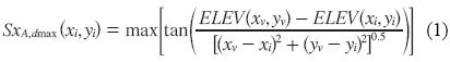
Where ELEV is the altitude of interest cell; A the azimuth of the search direction; (x_i, y_i) coordinates of the cell of interest; (x_v, y_v) the coordinates of the cells found in the same direction of prevailing wind and dmax is the maximum search distance.

The application of the upwind index for the Eastern Pyrenees was best correlated with snow depth at a prevailing wind direction of 220°. Empirically, the maximum distance of search vector was established at 300 m.

Finally, Pearson's correlation between each variable and snow depth was calculated to evaluate the relation between them with SPSS 16.0 statistical software.

3.3.2. Snow depth modeling

As previously mentioned, modeling of snow depth was achieved through the extrapolation of strip flight data. Existence of data for the whole area permitted validation of the final model.

A stepwise regression tree (SRT, Huang and Townshend, 2003) was used to model snow depth because it considers the non–linearity of dependent variables. This is the most important characteristic for modeling snow depth calculations (De'Ath and Fabricius, 2000; Huang and Townshend, 2003). The SRT method has been implemented by Loh (2002) and Loh et al. (2008) in the GUIDE algorithm (Loh, 2011) as an evolution of the classical tree classification proposed by Breiman et al. (1984).

The GUIDE algorithm was used for a stepwise regression tree. The independent topographical variables were used to explain snow depth (dependent variable). In a classical tree classification the assigned value for prediction is the mean of each node. Consequently, the range of predicted values is limited to the number of final nodes of the tree. Loh (2002) and Huang and Townshend (2003) propose a stepwise regression at each final node. The regression at each final node ensures a small and homogeneous sample size which implies a better accuracy of prediction and cartography. In this way, the prediction value is not limited to a mean on the final nodes (because a regression is made) and a range of values is permitted, making prediction more accurate. Pruning was made through 10 cross–validation iterations and the minimum sample size for each node was 7500 data points.

 

4. Results and discussion

4.1. LIDAR snow depth model validation

The aim of snow depth validation was to establish the RMSE of the snowpack and a feasible maximum value of snow depth. With these values the model was validated by removing negative and extreme positive snow depths. Validation was carried out on the snow depth map obtained from the subtraction of the LIDAR–generated DEMs.

4.1.1. Validation through field data

Despite the use of LIDAR for snow depth calculations (Fassnacht and Deems, 2005; Deems and Painter, 2006), few validations have been achieved with field data. Hopkinson et al. (2004) estimated that differences between LIDAR data and field measurements were around 19 %.

In this study there are many factors that affect the quality of results:

1. Despite efforts to increase efficiency in field work the validation data was limited to 74 points, which is probably insufficient to ensure data representativeness.

2. The field surface surveyed was uneven and rocky, resulting in biased field data. The variability of snow depth within 1 m² was high and the exact place where the snow probe was inserted is of great importance (even though the nested method for snow sampling was adopted during field work).

3. Snowpack conditions induce measurement errors. Presence of ice layers within the snowpack impeded the correct penetration of the snow probe.

4. Mountainous terrain induces GPS precision errors. Moreover, data acquisition in steep slopes coincided with areas where LIDAR techniques presented more deficiencies.

These factors resulted in unsatisfactory results which were therefore not considered when performing validation. Validation was therefore achieved with aerial photographs and profile making in accumulation areas.

4.1.2. Validation with aerial photographs.

Although only 74 point data were obtained through manual surveying, with the digitalization of snow–free control areas, a total of 680 000 data points were obtained, representing an area of 0.7 km² (2 % of the total study area).

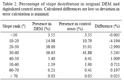
Since slope is the major source of error in LIDAR surveys, slope distribution at the control areas should be very similar and representative of the entire study area. The presence of higher slopes in control areas would mean an increment in the calculation error of snow depth. Table 2 shows all slope classes (every 10°) for the whole area and for the control areas. All ranges were well represented during digitalization so deviations in the error source were avoided.

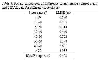
For comparison, Table 3 shows RMSE obtained for snow depth calculations in control areas (0 cm) from LIDAR data depending on different slope ranges. The results show that error increases with slope and that low snow accumulation in slopes of more than 60° also increases error. Thus we excluded these slopes in the final RMSE calculation. The final RMSE calculated value for control areas was 0.428 m.

4.1.3. Validation in snow accumulation areas

After subtraction of the DEM, the resulting snow depth presented extreme values that should be investigated. A total of 17 topographic profiles were made for this purpose, two of which are shown in Figures 6 and 7.

Both figures demonstrate how bare–earth and snowpack follow the same topographical trend, which implies that the snow depth values are correct measurements. The same analysis made on 17 profiles showed evidence that snow depth accumulations of up to 11 meters were valid in very specific topographical conditions, namely deep streams and wind–sheltered areas. During validation all values higher than 11 m were therefore considered erroneous and subsequently eliminated.

4.1.4. Validated snow map.

After the validation process a range of valid values was established and applied to the LIDAR snow model. This range lies between –0.428 m, corresponding to the RMSE calculated, and 11 m, from the profile analysis. A value of 0 m depth was assigned to measurements between –0.428 m and 0 m. The resulting snow model therefore ranges from 0 m to 11 m of snow depth (Figure 5).

4.2. Snowpack modeling

4.2.1. Snow and terrain parameters correlation

To select variables that best explained the distribution of snow over the pilot area, the Pearson correlation coefficient was calculated between topographical variables and snow depth. Figure 8 shows these correlation coefficients.

Major correlation was found with the upwind index (r = 0.447), and with curvature (r = –0.328). Surprisingly, there was no important correlation with altitude (r = 0.116), mainly due to specific distribution of snowpack over the study area. Greater snow accumulations were situated in wind sheltered areas and north facing slopes. In contrast, the wind produced snow–free surfaces at higher altitudes.

Another important factor which must be considered to fully understand correlation coefficients is that the LIDAR flight was carried out on March 27^th when melting had already begun.

Based on the Pearson correlation, slope and altitude were excluded from the SRT analysis due to their low correlation with snow depth.

4.2.2. Extrapolation of snow depth

The GUIDE algorithm (Loh et al., 2008) permitted a prediction of snow depth from one flight strip as pointed out in the methodology. The result of the modeling process was a classification tree composed of 19 final nodes (Figure 9).

The model was run recursively with different parameters (regression type, number of cross–validation iterations etc.) until reaching the optimum model presented. The best tree model is the one with the smallest number of final nodes. An excessive number of nodes results in the overestimation of the model. An example of the influence of the final number of nodes over the model adjustment is shown in Figure 10. The figure shows how an increasing number of final nodes implies an overestimation and erroneous adjustment of the model.

The final model, R²=0.44, is very significant due to the fact that we used a relatively high spatial resolution (5 m) and a great number of data was modeled (more than 1 million data points). Despite this, the RMSE was significant (0.69 m), and the model fit was very satisfactory for the study purpose (snow volume). The ultimate aim of the project was to evaluate water supplies stored as snow. In this sense, the difference in total snow volume is more important than snow depth accuracy. So if snow volume calculated from the validated LIDAR model (33.7 hm3 of snow) is compared to snow volume calculated from the extrapolated final model (33.9 hm³) the difference is only –1 %.

Authors such as Elder et al. (1998) have presented an R² of 0.68 with computations made on a 30 m resolution DEM. Afterwards, in parcels of 1 km², Erxleben et al. (2002) showed an adjusted R² of 0.298. López–Moreno and Nogués–Bravo (2006), with 106 data points for the entire Pyrenees, obtained an adjusted R² of 0.71 and, finally, Molotch et al. (2005) present values between 0.31 and 0.39 (after performing a residual interpolation procedure).

Figure 11 shows the final map result of extrapolation.The map reflects high spatial variability of snow depth, which is one of its most well known characteristics (Elder et al., 1995).

Other aspects to consider in the map analysis are: a) large accumulations in streams are only visible over 1900 m so the influence of curvature is restricted to high altitudes; b) the map shows south–facing slopes situated at lower heights without snow, which matches field observations; and finally c) north–facing areas which are topographically sheltered from wind show great snow accumulations and are also well represented in the final model.

In summary, the snow volume difference between the LIDAR model and extrapolated model was only –0.69 %. That result seems to validate the methodology and technique used in a wide area (38 km²) with a large number of data.

 

5. Conclusions

By using both LIDAR technology and the SRT extrapolation modeling technique, a precise cartography of snow depth distribution was obtained. Regression application at each final node together with a considerable amount of data obtained with LIDAR permitted good prediction values for snow depth and, more importantly, total amount of accumulated snow.

Several data validation methods were applied because field work results were less useful than expected. On the other hand, despite being a new solution, the use of aerial photographs during validation was demonstrated to be useful. At the same time, aerial photographs ensure a high data representativeness. Comparing topographic profiles, with snow and without snow, it was possible to establish a maximum limit in snow depth measurements. Application of more sophisticated techniques, such as geo–radar, to get data from snow depth accumulation areas and validation with more field data are challenges for research in the near future.

Finally, we point out that the next investigation efforts in Núria valley will be focused on studying snow water equivalent within the valley (this includes snow water equivalent sampling) and modeling basin with the installation of gauging stations and a comparison of modeled snow volume calculations with measured runoff.

 

Acknowledgements

The authors would like to thank all those who collaborated and all those in charge at the Vall de Núria ski resort for their courtesy. Further thanks to A. Winstral for providing the algorithm to calculate upwind index and to W. Loh for freely distributing his GUIDE algorithm. The authors are also grateful for the contributions made by, James R. Carr and N. Glenn, who kindly improved this paper by reviewing it.

 

References

Agència Catalana de l'Aigua (ACA), 2005, Memòria any 2005: Barcelona, Departament de Medi Ambient, Generalitat de Catalunya, 167 p.         [ Links ]

Breiman, L., Friedman, J.H., Olshen, R., Stone, C., 1984, Classification and Regression Trees: Belmont California, Wadsworth International Group, 358 p.         [ Links ]

Burrough, P.A., van Gaans, P., Macmillan, R.A., 2000, High–resolution landform classification using fuzzy k–means: Fuzzy Sets and Systems, 113, 37–52.         [ Links ]

Capel Molina, J.J., 2000, El clima de la península Ibérica: Barcelona, Editorial Ariel, 281 p.         [ Links ]

Cline, D., Elder, K., Bales, R., 1998, Scale effects in a distributed snow water equivalent and snowmelt model for mountain basins: Hydrological Processes, 12, 1527–1536.         [ Links ]

De'Ath, G., Fabricius, K., 2000, Classification and regression trees: A powerful yet simple technique for ecological data analysis: Ecology, 81, 3178–3192.         [ Links ]

Deems, J.S., Painter T.H., 2006, LIDAR measurements of snow depth: accuracy and error sources, in Proceedings of the 2006 International Snow Science Workshop: Telluride, Colorado, USA, International Snow Science Workshop, 330–338.         [ Links ]

Departament de Medi Ambient i Habitatge (DMAH), 1993, Mapa de cobertes del sòl de Catalunya, maps 217–2–2 and 217–2–1, scale 1:25.000: Barcelona, Centre de Recerca Ecològica i Aplicacions Forestals, Generalitat de Catalunya, 2 maps.         [ Links ]

Elder, K., Michaelsen, J., Dozier, J., 1995, Small basin modeling of snow water equivalence using binary regression tree methods, in Tonnessen, K.A., Williams, M.W., Tranter, M. (eds.), Biochemistry of Seasonally Snow–Covered Catchments: Wallingford, Oxfordshire, Reino Unido, International Association of Hydrological Sciences, 129–139.         [ Links ]

Elder, K., Rosenthal, W., Davis, R., 1998, Estimating the spatial distribution of snow water equivalence in a montane watershed: Hydrological Processes, 12, 1793–1808.         [ Links ]

Erxleben, J., Elder, K., Davis, R., 2002, Comparison of spatial interpolation methods for estimating snow distribution in the Colorado Rocky Mountains: Hydrological Processes, 16, 3627–3649.         [ Links ]

Fassnacht, S.R., Deems, J.S., 2005, Scaling associated with averaging and resampling of LIDAR–derived montane snow depth data, in Hellström, R., Frankenstein, S. (eds.), Proceedings of the 62nd Eastern Snow Conference, Waterloo, Ontario, Canada: USA, Eastern Snow Conference, 163–172.         [ Links ]

Hopkinson, C., Demuth, M., 2007, Using airborne LIDAR to assess the influence of glacier downwasting to water resources in the Canadian Rocky Mountains: Canadian journal of remote sensing, 32, 212–222.         [ Links ]

Hopkinson, C., Sitar, M., Chasmer, L., Gynan, C., Agro, D., Enter, R., Foster, J., Heels, N., Hoffman, C., Nillson, J., Sant Pierre, R., 2001, Mapping the spatial distribution of snowpack depth beneath a variable forest canopy using airborne laser altimetry, in Hardy, J., Frankenstein, S. (eds.), Proceedings of the 58th Eastern Snow Conference, Ottawa, Ontario, Canada: USA, Eastern Snow Conference, 253–264.         [ Links ]

Hopkinson, C., Sitar, M., Chasmer, L., Treitz., P., 2004, Mapping snowpack depth beneath forest canopies using airborne lidar: Photogrametric Engineering and Remote Sensing, 70, 323–330.         [ Links ]

Huang, C., Townshend, J.R.G., 2003, A stepwise regression tree for nonlinear approximation: applications to estimating subpixel land cover: International Journal of Remote Sensing, 24, 75–90.         [ Links ]

Institut Cartogràfic de Catalunya (ICC), 1996, Atles climàtic de Catalunya: Barcelona, Departament de Política Territorial i Obres Públiques Generalitat de Catalunya, 42 maps.         [ Links ]

Institut Cartogràfic de Catalunya (ICC), 2010, Webserver de les estacions de referència GPS (website): Barcelona, Institut Cartogràfic de Catalunya, available at <http://catnet–ip.icc.es/>         [ Links ].

Kaneta, S., Hatake, S., 2007, Snow depth distribution by airborne LIDAR data (on–line document): Noida, India GIS Dvelopment, available at <www.gisdevelopment.net/technology/survey/ma07131.htm>         [ Links ].

Kornus, W., Ruiz, A., 2003, Strip adjustment of LIDAR data, in Maass, H.G., Vosselman, G., Streilein, A. (eds.), Proceedings of the ISPRS working group III/3 workshop: Dresden, Germany, International Society of Photogrammetry and Remote Sensing (ISPRS),         [ Links ] .

Loh, W., 2002, Regression trees with unbiased variable selection and interaction detection: Statistica Sinica, 12, 361–386.         [ Links ]

Loh, W., Chen, C.W., Zheng, W., 2008, Extrapolation errors in linear model trees: ACM Transactions on Knowledge Discovery from Data, 1, 1–17.         [ Links ]

Loh, W., 2011, GUIDE Classification and Regression Trees (on–line algorithm): Madison, Wisconsin, University of Wisconsin–Madison, available at <www.stat.wisc.edu/~loh/guide.html>, accessed 17^th April 2011.         [ Links ]

López–Moreno, J., Nogués–Bravo, D., 2006, Interpolating snow depth data: a comparison of methods: Hydrological Processes 20, 2217–2232.         [ Links ]

López–Moreno, J., Vicente–Serrano, S.M., Lanjeri, S., 2007, Mapping snowpack distribution over large areas using GIS and interpolation techniques: Climate Research, 33, 257–270.         [ Links ]

Marchand, W.D., Killingtveit, A., 2001, Analyses of the relation between spatial snow distribution and Terrain Chacarcteristics, in Hardy, J., Frankenstein, S. (eds.), Proceedings of the 58th Eastern Snow Conference, Ottawa, Ontario, Canada: USA, Eastern Snow Conference, 71–84.         [ Links ]

Marchand, W.D., Killingtveit, A., 2005, Statistical probability distribution of snow depth at the model sub–grid cell spatial scale: Hydrological Processes 19, 355–369.         [ Links ]

Molotch, N.P., Colee, M.T., Bales, R.C., Dozier, J., 2005, Estimating the spatial distribution of snow water equivalent in an alpine basin using binary regression tree models: the impact of digital elevation data and independent variable selection: Hydrological Processes, 19, 1459–1479.         [ Links ]

Rosenthal, W., Dozier, J., 1996, Automated mapping of montane snow cover at subpixel resolution from the Landsat Thematic Mapper: Water Resources Research, 32, 115–130.         [ Links ]

Salomonson, V.V. , Appel, I., 2004, Estimating fractional snow cover from MODIS using the normalized difference snow index: Remote Sensing of Environment, 89, 351–360.         [ Links ]

Sangrà, J.M., 2008, Qui paga l'aigua? in Aigua: font de vida, font de risc. Informe 2008 de l'Observatori del Risc: Barcelona, Institut d'Estudis de la Seguretat.         [ Links ]

Servei Meteorològic de Catalunya (SMC), 2008, Butlletí climàtic de l'any 2007 (on–line document): Barcelona, Departament de Medi Ambient, published 13 February 2008, available at <www20.gencat.cat/docs/meteocat/Continguts/Climatologia/Butlletins%20i%20resums%20climatics/Butlletins%20anuals/2007/Butlleti_climatic_2007.pdf>         [ Links ].

Ulied, A. (coord.), 2003, Catalunya cap al 2020. Visions sobre el futur del territori: Barcelona, Departament de Presidencia, Generalitat de Catalunya, 160 p.         [ Links ]

Winstral, A., Marks, D., 2002, Simulating wind fields and snow redistribution using terrain–based parameters to model snow accumulation and melt over a semi–arid mountain catchment: Hydrological Processes, 16, 3585–3603.         [ Links ]

Winstral, A., Elder, K., Davis, R.E., 2002, Spatial snow modeling of wind–redistributed snow using terrain–based parameters. Journal of Hydrometeorology, 3, 524–538.         [ Links ]