Artículos

 

Kinematic source analysis of the 2003 Tecomán, México, earthquake (Mw 7.6) using teleseismic body waves

 

Análisis cinemático de la fuente del sismo de Tecomán 2003 (Mw 7.6), México, mediante ondas de volumen telesísmicas

 

Juan Martín Gómez–González¹*, Carlos Mendoza¹, Anthony Sladen², Marco Guzmán–Speziale¹

 

¹ Centro de Geociencias, Universidad Nacional Autónoma de México, Campus Juriquilla, Blvd. Juriquilla 3001, 76230 Querétaro, Qro., México. * E–mail: gomez@geociencias.unam.mx

² Tectonics Observatory, Division of Geological and Planetary Sciences, California Institute of Technology, Pasadena, California, USA.

 

Manuscript received: March 2, 2009.
Corrected manuscript received: January 8, 2010.
Manuscript accepted: April 11, 2010.

 

Abstract

We analyze the Tecomán, Colima, earthquake (Mw 7.6) of January 22, 2003, one of the major seismic events that has occurred in the Colima–Jalisco region, México, during the last 100 years. We describe its rupture process by a classical waveform modeling of teleseismic body waves. A point source inversion indicates a shallow underthrust event (25 km); its fault plane is defined by a strike of 278°, a dip of 27°, and a rake of 78°. The source time function (STF) has a total duration of about 22 s and shows a relatively simple time history. The main moment release is preceded by a small onset of about 6.6 sec, located 17 km south of the main moment release. This precursor is associated with an initial rupture velocity of about 2.6 km/s. Slight azimuthal variations of relative source time functions (RSTF) indicate a weak directivity, probably produced by a bilateral asymmetrical rupture oriented NNE–SSW. The RSTFs confirm that the Tecomán earthquake is composed of three subevents that mainly ruptured down–dip. A finite line–source analysis along the strike and dip also confirms the orientation of the rupture propagation and shows the wide range of apparent rupture velocities along the fault. The Tecomán earthquake is an interesting case of a well–recorded event, with good quality data, but with results that are poorly constrained, which affects the uncertainty of several parameters, like directivity and hypocenter depth.

Keywords: Body waves, earthquake–source mechanism, fault plane solution, seismology, source time function, waveform analysis.

 

Resumen

Se analiza el sismo de Tecomán, Colima (Mw 7.6), del 22 de enero de 2003. Este es uno de los sismos más grandes ocurridos en la región de Colima–Jalisco, México, en los últimos 100 años. Se describe su proceso de ruptura mediante el modelado de ondas de cuerpo telesísmicas. La inversión de fuente puntual indica un evento somero de falla inversa de bajo ángulo (profundidad del centroide = 25 km), con un rumbo del plano de falla de 278°, un echado de 27° y un ángulo de deslizamiento de 78°. La función temporal de la fuente (STF) es relativamente simple, con una duración aproximada de 22 s. La liberación principal del momento sísmico fue precedida por una pequeña fase de aproximadamente 6.6 s de duración, localizada 17 km hacia el sur de la principal distribución de momento sísmico. Este precursor está asociado con una velocidad de ruptura inicial cercana a 2.6 km/s. Las leves variaciones azimutales de la función temporal de la fuente relativa (RSTF) indican una directividad débil, producida probablemente por el carácter bilteral asimético de la ruptura orientada NNE–SSW. El proceso de ruptura está compuesto por tres subeventos que rompieron a lo largo del plano del echado, hacia la base de la falla. Para verificar esta distribución llevamos a cabo un análisis de fuente finita de una franja sobre la superficie de la falla paralela al rumbo y otra al buzamiento. Este análisis también permite visualizar de forma rápida el intervalo de velocidades aparentes de ruptura a lo largo de la falla. El sismo de Tecomán es un caso interesante de un evento bien registrado, con datos de buena calidad, pero con resultados pobremente restringidos, lo que influye en la incertidumbre de varios parámetros, como la directividady la profundidad del hipocentro.

Palabras clave: Ondas de volumen, mecanismo de la fuente sísmica, solución de plano de falla, sismología, función temporal de la fuente, análisis de la forma de onda.

 

1. Introduction

The Tecomán, Colima, México, earthquake (Mw 7.6) of January 22, 2003 occurred near the triple junction of the Cocos, Rivera, and North American plates and ruptured a portion of the western half of El Gordo Graben (Figure 1). This tectonic feature is part of the gap between the aftershock areas of the January 30, 1973 (Ms 7.6) and the October 9, 1995 (Mw 8) Colima–Jalisco earthquakes (Courboulex et al, 1997; Mendoza and Hartzell, 1999). The earthquake is one of six large events that have occurred in the last 100 years in the Colima–Jalisco region (Singh et al., 2003). Here, the historical seismicity is characterized by shallow thrust events (Figure 2). The Global Centroid Moment Tensor (CMT) Project located the centroid of the Tecomán earthquake at 103.90°W, 18.86°N (2:06:48.9 GMT), at a depth of 26 km (Figure 2). The local Red Sismológica del Estado de Colima (RESCO) network, operated by the University of Colima, obtained a hypocentral depth of 10 km. This depth is similar to that determined by the Mexican Servicio Sismológico Nacional (SSN) network (9.5 km). Most of the aftershocks recorded during the first week delimited a relatively small area (Figure 1) located toward the western edge of the Southern Colima Rift (SCR) (Schmitt et al., 2007) that partially overlaps the eastern edge of the longer aftershock area of the October 9, 1995 Colima–Jalisco earthquake (Singh et al., 2003). The 1995 Colima–Jalisco and the 2003 Tecomán events started at opposite sides of the western edge of the SCR. Most of the Tecomán aftershock locations are concentrated in the upper 10 km of the crust (Schmitt et al., 2007). Based on this information Núñez–Cornú et al. (2004) proposed that the Tecomán earthquake was produced by a continental intraplate reverse fault in a plane with an orientation of N80°E and a dip of 40°. Eventhough, Rodríguez–Lozoya et al. (2007) obtained similar depths for most of the aftershocks they located the mainshock along the bend of the subducted slab, suggesting an interplate earthquake.

Singh et al. (2003) studied the Tecomán earthquake by carrying out a single station analysis of ground motion data. They modeled the deformation by considering an average dislocation of 2 m over a fault area of about 40 x 40 km². They proposed a unilateral rupture towards the NNE, finding it compatible with the horizontal deformation observed at the Manzanillo Global Positioning System (GPS) site. Yagi et al. (2004) found a similar rupture orientation mainly concentrated along the dip, but their 2–D waveform modeling suggested a bilateral rupture. They carried out a joint inversion of teleseismic body waves and near–source data and proposed a narrower rupture area (40 x 70 km²), an average dislocation of 3 m with a constant rupture velocity, and a source time function (STF) of 30 s. Schmitt et al. (2007) estimated a dislocation of 2 m by using coseismic displacements and aftershock information from GPS sites.

The direction of rupture propagation during the Tecomán earthquake is almost perpendicular to that of the 1995 Colima–Jalisco earthquake, which was towards the NW along the strike (Courboulex et al., 1997; Mendoza and Hartzell, 1999). Schmitt et al. (2007) confirmed the rupture direction along the dip by using near–term post seismic measurements. In addition, the results of Yagi et al. (2004) and Schmitt et al. (2007) indicate that the Tecomán earthquake can be explained by a bilateral rupture. This mechanical process is not common worldwide (McGuire et al, 2002), especially for shallow subduction earthquakes with bilateral rupture along the dip (Hartog and Schwartz, 1996; López and Okal, 2006). McGuire et al. (2002) analyzed 25 major shallow earthquakes (Mw > 7) occurring between 1994 and 1999 for different tectonic environments and found a predominance (80%) of unilateral rupture with respect to bilateral rupture, with most events showing a preferred rupture along the strike. This percentage seems to be consistent with known earthquakes at the Mexican subduction zone, where few bilateral events have been reported. The Ms 7.3 Playa Azul earthquake of October 25, 1981 is the most recent event showing up–dip and down–dip contributions (Mendoza, 1993).

In this paper we carry out waveform modeling in order to compute the basic parameters of the source of the Tecomán earthquake. Complementary analyses are used to reevaluate two parameters: the orientation of the rupture propagation and its rupture velocity. In order to learn more about these parameters we carry out a directivity analysis that enables us to visualize the azimuthal variations of the relative source time functions. The other analysis is line–source modeling, which provides the range of rupture velocities along the strike and dip and helps to confirm the STF duration. The Tecomán earthquake is an example of how a well–recorded seismic event with good–quality data yields poorly constrained results due probably to the nature of the source.

 

2. Seismotectonic setting

The Colima–Jalisco region is located at the triple junction of the North America (NOAM), Rivera (RIVE), and Cocos (COCO) plates (Figure 1). The RIVE and COCO plates subduct below the NOAM plate and it is in this portion of the Middle America Trench where several large earthquakes have occurred (Singh et al., 2003). The epicenter of the Tecomán earthquake was located in the El Gordo graben, an important tectonic feature where the downgoing RIVE and COCO plates probably decouple (Bandy et al., 1995; Bandy et al., 2000). The deformed region between these plates is characterized by NNE–SSW trending thrust faulting (Pardo and Suárez, 1995). The convergence rate of the RIVE–NOAM and COCO–NOAM plates are similar in front of the Southern Colima Rift, about 5 cm/yr (Kostoglodov and Bandy, 1995). The age of the oceanic plates at the trench is about 10 Ma (Klitgord and Mammerickx, 1982; Atwater and Severinghaus, 1989). Pardo and Suárez (1993; 1995) suggested that the maximum depth of seismogenic coupling for the RIVE plate could reach ~40 km, while in the case of the COCO plate, this depth could be shallower than ~25 km. Most earthquakes within the subducted RIVE and COCO plates have thrust–fault focal mechanisms (Figure 2). Singh and Mortera (1991) analyzed several thrust earthquakes along the coupled interplate contact in southern México and found that different rupture modes and source complexity are probably related to variations in the strength of coupling along the plate interface, but not to the geometry of the subduction or to the depth extent of the coupled interplate zone. Schmitt et al. (2007) suggest a limit to the area of potential slip and hence on the rupture extent during future large earthquakes in the region.

 

3. Precursory phase

The Tecomán earthquake was preceded by a precursory phase, which was observed on local data (Singh et al, 2003). This precursor can also be observed on teleseismic data (Figure 3A). This kind of short subevent has been observed for several earthquakes (Bezzeghoud et al, 1986; Ihmlé and Jordan, 1994; Campos, 1995; Fuenzalida, 1995, Gómez et al, 1997). The precursors occur in a short time interval, and sometimes they just precede the main moment release and may be related to the rupture process (Iio, 1992; Ellsworth and Beroza, 1995; Beroza and Ellsworth, 1996; Hartog and Schwartz, 1996; Umino et al, 2002).

Even though the quality of the seismic data is good, identification of precursory phases is still difficult. Extreme care is required in order to identify precursors, separate them from the main moment release and distinguish them from other effects like instrumental or environmental noise. These phases have received more attention in the literature in the last 20 years due to the improvement of physical–rupture and nucleation models and their analysis. These contributions have provided important information on the interpretation of nucleation phases (Iio, 1992; Ellsworth and Beroza, 1995). These features are sometimes more readily observed in the near field, where source analyses have proved the existence of precursory phases for different earthquake magnitudes (Iio, 1992; Ohnaka, 1992, 1993; Abercrombie and Mori, 1994; Ellsworth and Beroza, 1995). Other precursory teleseismic phases have also been observed at lower frequencies for large earthquakes (Kanamori, 1989; Jordan, 1991; Ihmlé et al, 1993; Ihmlé and Jordan, 1994).

For the Tecomán earthquake, Singh et al. (2003) identified a small phase preceding the P–wave onset based on a fine inspection of accelerograms. This precursor is also observed on several teleseismic broadband P–wave seismograms. In order to obtain information about the location and duration of the Tecomán precursory phase relative to the main moment release, we have carried out a directivity analysis (Hartog and Schwartz, 1996). We picked the precursor P–wave onsets directly from velocity seismograms, while onsets of the main moment release were clearer on the displacement signals (Figure 3A). We considered only those records where the precursor is more clearly determined.

The estimation of the time and place where the precursory energy supposedly initiated is obtained by solving the following equation: t = t₀ – X Γ, where Γ = p cos (φ – φ₀), which relates the apparent rupture duration (t) to the actual source duration of the precursor (t₀) and the direction of rupture propagation (φ₀). X is the length of the rupture, p is the ray parameter, and p is the azimuth to the station. The azimuth yielding the most linear behavior of the time shifts, in the precursor versus the directivity parameter Γ, is identified as the actual rupture direction. Corresponding values of t₀ and X reveal the temporal and spatial finiteness of the rupture associated with the precursory phase (Figure 3B). This analysis assumes a unilateral propagation; however it is useful to find the relative spatial position of the main moment release. Figure 3C shows the variations of the linear correlation coefficient as a function of azimuth and suggests that the main rupture started about 6.6 ± 1.15 seconds later and 17 ± 3.3 km towards the north with respect to the precursor. From these parameters, we can deduce an initial rupture velocity of about 2.6 km/s.

The uncertainty in picking the initial P–wave arrivals results in uncertainties in obtaining the corresponding correlation coefficient. There is also a large uncertainty in visually picking the end of the precursory phase. Instead of measuring the pulse width on each seismogram, Warren and Shearer (2006) developed a method to systematically estimate the pulse width using the slope of their log spectra. However, the quality of the picks is degraded when the rupture is more complex, as in the case of bilateral rupture.

 

4. Body waveform modeling

We carried out a source analysis by inverting the body–wave teleseismic signals. The records were obtained from the IRIS Data Management Center and were provided by several incorporated networks (FDSN, GEOFON, Geoscope, IDA, GTSN, UI, USGS). We use the classical linear algorithm of Nábélek (1984; 1985), which is based on a point source approximation. The method searches for basic source parameters (strike, dip, rake, centroid depth, scalar moment and rupture duration). Depending on the size and complexity of the earthquake, the source can be parameterized either as a single point source or as an event consisting of several point sources (subevents) separated in time and space. Since the relationship between the theoretical model and the source parameters is non–linear, the minimization is done by an iterative procedure based on a gradient method with a positivity constraint. The algorithm minimizes the waveform differences between observed and computed seismograms by calculating the sum of the square of the residuals.

The Source Time Function (STF) is parameterized as a series of overlapping trapezoids (Nábélek, 1984), each of them resulting from the convolution of two boxcar functions of equal duration T(t – τ_k) = B_Δτ (t) * B_Δτ^r (t). For each subevent Δτ represents the rise time, and the other Δτ^r the rupture duration (Lay and Wallace, 1995), where τ_k= Δτ (k –1), k=1, nτ, and m is the number of trapezoids. The number of time function elements and their durations are chosen a priori.

Seismograms contain many phases, or arrivals, corresponding to different travel paths. The Nábélek (1984) algorithm uses direct and depth phases (P, pP, sP, S, pS, and sS) for waveform modeling, with the source information contained in the first seconds of the seismograms. We invert a time window of 80–second duration of the vertical P and transverse SH wave displacements. In order to avoid multipathing and upper–mantle triplications we use stations located at epicentral distances of 30° < Δ_p < 90° and 34° < Δ_SH < 87°. At these distances core reflections are not expected to affect the waveform modeling because amplitudes are less significant due to the small impedance contrast at the core–mantle boundary (Storchak et al., 2003; Crotwell et al, 1999). In addition, these phases are well differentiated with respect to direct waves along the majority of the path.

Teleseismic body waves are relatively easy to model using synthetic seismograms due to the homogeneity of the earth's mantle and the fact that observations are made at a great distance from the source. The wave packets can be approximately characterized by a single ray parameter (Langston and Helmberger, 1975; Bouchon, 1976). This approximation implies that out of all the rays of up and down–going P and S waves that depart from the source, only four of them contribute to the body wave seismogram (Nábélek, 1984). In order to calculate the teleseismic body wave Green's function, the algorithm splits the calculation into two parts: the contributions from the crustal and free–surface effects in the source and receiver regions, and the contribution from the mantle. Because of the homogeneity of the mantle, this portion of the propagation path can be accounted for by considering only geometrical spreading (Bullen, 1963), anelastic attenuation (Futterman, 1962) and travel time.

4.1. Point source approximation

Despite the presence of the precursory phase on the January 22, 2003, Tecomán earthquake (Mw 7.6), the teleseismic waveforms look relatively simple. Thus, for simplicity, we consider the precursory phase as a part of the main moment release during the body waveform modeling. For inverting the double couple source parameters, we adopted the epicentral location of the centroid reported by the Global CMT Project (Table 1). We assume a 2–s rise time and use ten overlapping triangles of 2 s half–duration to define the possible maximum STF duration, which is allowed to take any arbitrary shape.

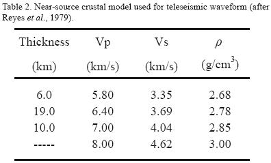
Anelastic attenuation is assumed constant for periods longer than t*, where we consider t* = 0.7 s and t* = 4 s for P and SH waves, respectively. The effects at the receiver are assumed negligible and the response is mostly controlled by the source radiation pattern at the near source structure. Green's functions are computed from a stratified velocity model (Table 2) based on the crustal structure of Reyes et al. (1979). For the receivers, a simple half–space model is used (Vp = 6.4 km/s, Vs = 3.69 km/s, ρ = 2.8 g/cm³ and a Poisson ratio of 0.25). Instrument responses are removed and the seismograms are filtered using a third–order Butterworth filter with a band pass from 0.01 Hz to 1.0 Hz.

The present worldwide station coverage and the quality of the signals enable us to carry out waveform inversions of P waves only. However, when the fault plane is not fixed, P and SH waves complement each other and together constrain the fault plane orientation. In addition, by adding SH waves we avoid misdeterminations of the fault plane, especially for shallow dip angles, where the slip vector orientation is poorly constrained. Figure 4 shows the comparison between observed and synthetic waveforms. The quality of the waveform fits, even for southward P–wave nodal stations (Figure 4A; PTCN and RPN), indicates that the Tecomán earthquake is well represented by a point source, at least at the periods analyzed here.

The majority of the stations remain in the tensional quadrant of the obtained focal mechanism. The angle of the southern dipping plane is practically constrained by stations PTCN and RPN. The fault plane solution is also well constrained due to the contribution of SH waves (Figure 4B), since their radiation pattern is orthogonal to that of the P waves. The distribution of polarities does not permit a shallower dipping angle (Figure 4A), such as that determined by HRV (12°) or the USGS (10°), nor does it allow the greater angle of 41° obtained by Núñez–Cornú et al. (2004) from local data.

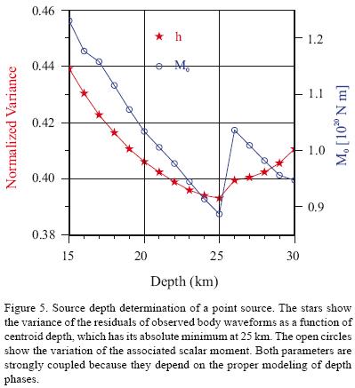
The geometry of the northern–dipping plane agrees well with the regional subduction characteristics of the Colima–Jalisco region (Figures 1 and 4). We chose this plane to represent the fault, corresponding to an underthrust solution defined by a strike (φ) of 278°, a dip (δ) of 27°, and a rake (λ) of 78° (Table 1). The best centroid depth is 25 km (Figure 5), corresponding to an STF duration of about 22 s and a scalar moment of 0.89 x 10²⁰ N m (Table 1). The centroid depth is similar to that reported by Yagi et al. (2004) and the Global CMT Project. Differences in depth relative to other reported solutions are due to differences in the types of data and the methods used.

4.2. Analysis of single relative source time function

Singh et al. (2003) proposed that rupture propagated initially toward the north from an analysis of local data. From a finite–fault analysis, Yagi et al. (2004) found that propagation occurred mainly along the dip, although the rupture behavior is bilateral. Then the next step is to examine the orientation of the rupture. Normally, the preferred propagation results in a directivity effect on waveform signals for a finite rupture length, where the radiated pulse duration varies directly as a function of azimuth and inversely to its amplitude (Stein and Wysession, 2003). Thus, directivity is useful to confirm the fault plane and to study the rupture propagation. However, the single average STF resulting from contributions of all the signals used in the point–source waveform inversion does not allow us to observe directivity effects. Another option is to obtain single–station STFs, which is equivalent to a point–source deconvolution for a single station (Kikuchi and Kanamori, 1982; Bezzeghoud et al., 1986). In this paper, each single STF is called a relative source time function (RSTF) in order to avoid confusion with the average STF.

In order to obtain the RSTFs, we fix the fault plane solution to that obtained in the previous point source analysis (φ=278°, δ=27°, λ=78°, and h = 25 km) and use the same inversion parameters as in the teleseismic body wave inversion: a time window of 80 s, a rise time of 2 s, and ten overlapping triangles of 2 s half–duration. Again these triangles are allowed to take any arbitrary shape to define their own possible maximum duration.

The set of RSTFs allows a qualitative evaluation of directivity. The individual RSTF should be shorter with high amplitude toward the direction of rupture propagation and should have a longer duration and smaller amplitude in the direction opposite of propagation (Stein and Wysession, 2003). The individual distribution of RSTFs obtained for the Tecomán earthquake is shown in Figure 6.A. Most of the RSTFs are composed of three pulses, with the first pulse being short relative to the main moment release. This short contribution is clearly observed as a left "shoulder" of the RSTF in almost all stations (YSS, PET, ADK, TIXI, BILL, FFC, KEV, SJG, RCBR, CPUP, LPAZ, NNA, and TRQA). This short contribution probably includes the precursory phase. The second pulse represents the main moment release and has a duration between 10 s and 15 s. Finally, the third pulse has an average duration of 5 s and appears beyond 13 s. At several stations, this third pulse immediately follows the end of the main moment release, especially for stations toward the north (COR, FFC, SFJ, and PAL). In some other cases, it appears isolated (YSS, PET, ADK, TIXI, BILL, COLA, KEV, RUE, CART, SJG, and EFI). The durations of the RSTFs range from 13 to 22 s. The length of the RSTFs at stations PTCN and RPN seem to be longer with respect to neighboring stations; however, these RSTFs are not as reliable because the stations are located near the nodal plane.

The variation of RSTFs seems to contradict the definition of directivity. If the propagation occurred toward the north, then the respective RSTFs should have shorter durations and greater amplitudes. However, the durations are long, of about 20 s, even though the amplitudes are high. Besides, towards the south, some durations are shorter than 15 s and have small amplitudes, except for the nodal stations, which have longer durations. By considering only the durations of the RSTFs, the propagation should have occurred toward the south. This inconsistency with respect to the definition of directivity could be related to asymmetrical rupture propagation because the eastern and western stations behave differently than the northern and southern stations. These effects could be due to the bilateral nature of the rupture along the dip. In addition, the three pulses observed at the majority of the RSTFs could be related to the three rupture stages described by Yagi et al. (2004). Figure 6.B shows the single waveform fits for each station.

4.3. Line–source analysis

A more complete description of the source behavior can be provided by a line–source analysis, which can be used to discriminate between a unilateral and a bilateral rupture. Also, it can provide more detailed information on the rupture velocity. Thus, we have carried out a line–source investigation by considering rupture propagation along a one–dimensional fault. The method is based on the 2–D finite–fault inversion procedure of Hartzell and Heaton (1983) but uses a single strip of subfaults to parameterize the fault. Mendoza and Hartzell (1999) used this parameterization to explore variations in rupture velocity for the 1995 Colima–Jalisco earthquake. Yagi et al. (2004) tested rupture velocities in the range of 2.5 to 4.5 km/s, and found that a constant rupture velocity of 3.5 km/s could explain the rupture process of the Tecomán earthquake. The appropriateness of this constant propagation can be examined with a line–source parameterization.

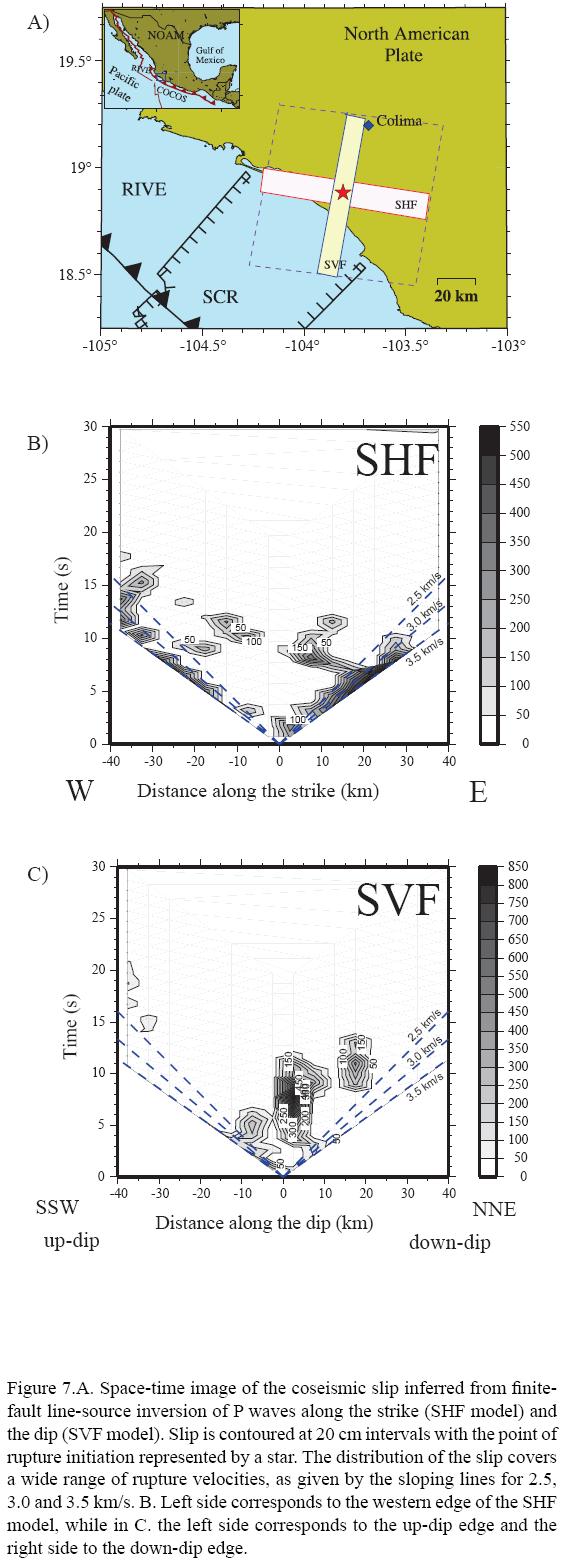
We use two different long narrow faults that allow variable rupture times over a broad time interval (Figure 7.A); this strategy allows us to examine variations in the rupture velocity for a unidirectional source. The faults are perpendicular to each other and are oriented in the direction of the strike and dip of the fault geometry determined from point–source waveform modeling (Table 1). The first model corresponds to a strip fault oriented almost E–W along the strike, model SHF (Figure 7.B), and the second fault is aligned almost N–S along the dip, model SVF (Figure 7.C). Both models have a maximum length of 80 km and are subdivided into sixteen 5 km x 5 km subfaults. The fault length is set to accommodate rupture velocities as high as 3.5 km/s based on the STF duration of 22 s obtained from waveform modeling.

Point sources are then distributed uniformly across each subfault using 1 km spacing. The fault is embedded in the crustal structure of Table 2, and subfault synthetic waveforms are computed at all stations by summing the response of each point source (Green's function) delayed by the time required for rupture to propagate at a velocity of 3.5 km/s from the hypocenter. As will be seen below, this value corresponds to an upper limit on the allowed rupture velocity. Green's functions are computed using the generalized ray summation technique described by Langston and Helmberger (1975) assuming a 1–s source–time function for each point source. The Green's functions incorporate internal reflections and mode conversions within the layered structure. Contributions of pP and sP phases are also included. The crustal attenuation value and the bandpass filter are the same as those used in the point source inversion.

The subfault synthetics are placed end–to–end to form an m x n matrix A, where m is the total number of data points for all stations and n is the number of subfaults. The observed data records are similarly joined in a data vector b to construct a system of linear equations of the form Ax=b that is solved for x, a vector that contains the subfault slips required to reproduce the observations. In the actual inversion, however, multiple consecutive rupture pulses are used to simulate dislocation over a broad time interval. This is done by successively lagging by 1–s intervals the subfault synthetics calculated assuming a 1–s rise time. The number of times that the synthetics are lagged represents the number of rupture pulses considered. This allows slip contributions at times later than the specified rupture velocity. For our line–source analysis, we use twenty 1–s time intervals to discretize the rise time on each subfault. The inversion thus provides subfault–slip amplitudes for each of the 20 time intervals following the passage of the 3.5 –km/s rupture front. A tomographic image of the earthquake rupture process can then be obtained by plotting the slip contributions along the length of the fault as a function of time. A more detailed description of this line–source inversion procedure is given by Mendoza and Hartzell (1999).

Figures 7.B and 7.C show the space–time distribution of coherent patterns of coseismic slip resulting from the line source inversion of P waves. Slip contributions of each subfault are contoured as a function of rupture time along the length of the fault. For the strip SHF there are two branches of constant propagation of rupture toward the east and west with respect to the hypocenter (Figure 7.B). The slip amplitude is greater towards the east and we observe that rupture velocity ranges mainly from 2.5 to 3.5 km/s. These variations make it difficult for point–source waveform modeling to obtain a reliable estimation of rupture velocity. The range of rupture velocities of Figure 7.B indicates that a single average value does not represent correctly the rupture process of Tecomán earthquake.

For the fault strip along the dip (SVF model) the left side of the horizontal axis (–40 km) in Figure 7.C corresponds to the uppermost edge of the fault strip, and the right side corresponds to the lowermost edge. The slip seems to be concentrated around the hypocenter, with an additional contribution towards the north (Figure 7.C). This position is relative, because the method projects 2–D distributions over the fault plane toward a line parallel to the strip of the fault. The slip distribution can be mainly associated with an updip–downdip rupture (Figure 7.C), similar to the results obtained by Yagi et al. (2004). The temporal distribution of slip (Figures 7.B and 7.C) gives a maximum rupture duration of 21 s, which is almost identical to the STF obtained by point source modeling. This STF duration is shorter with respect to the 30–sec duration obtained by Yagi et al. (2004); differences could be due to differences in methodologies.

 

5. Discussion

By using a classical point source waveform analysis we retrieved the basic source parameters of the Tecomán (Mw 7.6), Colima México, earthquake. One of the challenges for this shallow subduction event is to demonstrate the existence of a precursory phase and to characterize it correctly. If this precursory phase is not clearly present in the teleseismic P waveforms, then it is also not clear in the relative source time functions because of its substantially lower energy.

The method for locating the precursory phase works properly for unilateral rupture, finding its relative position with respect to the main moment release. Picking the end of the precursor is largely uncertain; in order to reduce this difficulty, precursor onsets were picked from the velocity traces, while the onsets of the main moment release were clearer on the displacement traces. Only records for which the P wave onset could be unambiguously determined were included in this analysis. The method does not distinguish the nature of the precursory energy; that is, it could be a nucleation phase or a foreshock related to the mainshock.

Azimuthal variations in the RSTFs provide information about the propagation direction but do not resolve the absolute location of moment release or the smaller scale features of the rupture process, particularly those preceding the main rupture, which are obscured by the deconvolution process. Our analysis suggests that the low energy onset is located just south of the area where most of the moment was released during the Tecomán earthquake.

The identification of directivity features was another challenge because the observations seem to contradict the definition of directivity. This inconsistency could be explained by an asymmetrical rupture propagation, which suggests the possibility that the earthquake occurred as a bilateral rupture along the dip, which has been proposed by other authors. This bilateral behavior could affect the observed directivity effects.

Even though a 2–D analysis provides a more complete description of the rupture process, new insight about the space–time distribution of rupture can be obtained from the line–source inversion of P waves. This method shows higher amplitudes toward the east, where the rupture velocity ranges from 2.5 to 3.5 km/s. These observations make it difficult for more simple methods to obtain a reliable estimation of the apparent rupture velocities. Therefore, an important conclusion is that a single rupture velocity does not accurately represent the rupture process of the Tecomán earthquake. For the second fault strip along the dip, SVF model (Figure 7.C), slip is concentrated around the hypocenter with an additional small contribution towards the north. The slip distribution can be mainly associated with an up dip–down dip rupture, similar to the results obtained by Yagi et al. (2004).

Finally, none of the analyses conducted here enable us to identify the physical conditions that resulted in this along–dip rupture. Additional studies are needed to know whether the elevated stress field associated with the propagating rupture front grows large enough to trigger failure of a possibly more strongly–coupled region down–dip. Scholz (1994) proposed that during dip–slip faulting process, subduction thrust events tend to nucleate near the down–dip end of the rupture zone. In addition, in the case of unilateral rupture the energy frequently propagates up–dip. A more complicated situation occurs for bilateral rupture along the dip. McGuire et al. (2002) consider that rupture propagation can be possible either up– or down–dip when elastic structures surrounding subducting zones are approximately two–dimensional and variations along strike are small. When large thrust events rupture the interface between the upper mantle and the more compliant subducting sedimentary layers, a down–dip rupture propagation would be favored. This possibility does not necessarily exclude the unilateral rupture explanation of Scholz (1994).

 

6. Conclusions

We obtained the basic geometrical characteristics of the January 22, 2003 Tecomán, earthquake (Mw 7.6), which corresponds to a shallow underthrust event. The duration of the STF obtained by point source approximation (22 s) is similar to that obtained by the line source analysis. However both are shorter with respect to the 30–s duration reported by the 2–D method (Yagi et al., 2004), possibly due to differences in methodology. Our STF duration is related to a scalar moment that is in good agreement with that of Schmitt et al. (2007), obtained by GPS analysis, but that is smaller with respect to the CMT solution obtained using long–period mantle waves.

We explored a precursory phase, which is located south of the hypocenter. The results of the line–source analysis coincide with the RSTF results and indicate that rupture is composed mainly by three subevents; the first onset is located SSW of the hypocenter, while the other two subevents are located to the NNE, with all of them distributed along the dip. These long narrow fault models show that a single average value cannot represent the time–space distribution of the source.

Our results agree with published results, which indicate that the Tecomán earthquake was controlled by an asymmetrical bilateral rupture with most of the scalar moment released down–dip. This distribution is probably responsible for the weak directivity observed on the teleseismic signals. In addition, more Mexican earthquakes must be analyzed in order to examine how frequently down–dip rupture occurs in the region. The Tecomán earthquake is an example of a well recorded event, with good quality data, that provides poorly constrained results

 

Acknowledgments

This work was funded by CONACyT grant J32466–T, and DGAPA–UNAM grants IN116399 and IN102102. Data were retrieved from SSN, IRIS, USGS, and the Global CMT Project databases. Signal processing was performed by using SAC (Tapley and Tull, 1991). Figures were made by using GMT software (Wessel and Smith, 1998). CGEO contribution No. 1230.

 

References

Abercrombie, R.E., Mori, J., 1994, Local observations of the onset of a large earthquake: 28 June 1992 Landers, California: Bulletin of the Seismological Society of America, 84, 725–734.         [ Links ]

Atwater, T., Severinghaus, J., 1989, Tectonic maps of the northeast Pacific, Plate 3C, in Winterer, E.L., Hussong, D.M., Decker, D.W. (eds.), The Eastern Pacific Ocean and Hawaii – The Geology of North America: Boulder, Colorado, Geological Society of America, 15–20.         [ Links ]

Bandy, W., Mortera–Gutierrez, C., Urrutia–Fugugauchi, J., Hilde, T.W.C., 1995, The subducted Rivera–Cocos plate boundary: Where is it, what is it, and what is its relationship to the Colima Rift?: Geophysical Research Letters, 22, 3075–3078.         [ Links ]

Bandy, W.L., Hilde, T.W.C.,Yan, C.Y., 2000, The Rivera–Cocos plate boundary: Implications for Rivera–Cocos relative motion and plate fragmentation: Geological Society of America Special Papers, 334, 1–28.         [ Links ]

Beroza, G.C., Ellsworth, W.L., 1996, Properties of the seismic nucleation phase: Tectonophysics, 261, 209–227.         [ Links ]

Bezzeghoud, M., Deschamps, A., Madariaga, R., 1986, Broad–Band Modeling of the Corinth, Greece Earthquake of February and March 1981: Annales Geophysicae, 4, 295–304.         [ Links ]

Bouchon, M., 1976, Teleseismic body wave radiation from a seismic source in a layered médium: Geophysical Journal Of the Royal Astronomical Society, 47, 515–530.         [ Links ]

Bullen, K.E., 1963, An Introduction to the Theory of Seismology: New York, USA, Cambridge Umversity Press, 381 p.         [ Links ]

Campos, J., 1995, La rupture sismique et ses environnements tectoniques: Paris, France, Université Paris VII, Ph.D. Thesis, 199 p.         [ Links ]

Courboulex, F., Singh, S.K., Pacheco, J.F., Ammon, C.J., 1997, The 1995 Colima–Jalisco, Mexico, earthquake (Mw 8): A study of the rupture process: Geophysical Research Letters, 24, 1019–1022.         [ Links ]

Crotwell, H.P., Owens, T.J., Ritsema, J., 1999, The TauP Toolkit: Flexible seismic travel–time and ray–path utilities: Seismological Research Letters, 70, 154–160.         [ Links ]

Ellsworth, W.L., Beroza, G.C., 1995, Seismic evidence for an earthquake nucleation phase: Science, 268, 851–855.         [ Links ]

Engdahl, E.R., Van der Hilst, R.D, Buland, R.P., 1998, Global teleseismic earthquake relocation with improved travel times and procedures for depth determination: Bulletin of the Seismological Society of America, 88, 722–743.         [ Links ]

Fuenzalida, H.A., 1995, Étude de sources de séismes complexes par inversion des ondes de volume (large–bande) dans la region du Caucase: Strasbourg, France, Université Louis Pasteur de Strasbourg, Ph.D. Thesis., 202 p.         [ Links ] .

Futterman, W.I., 1962, Dispersive body waves: Journal of Geophyical Research, 67, 5279–5291.         [ Links ]

Gómez, J.M., Bukchin, B., Madariaga, R., Rogozhin, E.A., Bogachkin B., 1997, Rupture process of the 19 August 1992 Susamyr, Kyrgyzstan, earthquake: Journal of Seismology, 1, 219–235.         [ Links ]

Hartog, J.R., Schwartz, S.Y., 1996, Directivity analysis of the December 28, 1994 Sanriku–Oki earthquake (Mw7.7), Japan: Geophysical Research Letters, 23, 2037–2040.         [ Links ]

Hartzell, S.H., Heaton, T.H., 1983, Inversion of strong ground motion and teleseismic waveform data for the fault rupture history of the 1979 Imperial Valley, California, earthquake: Bulletin ofthe Seismological Society of America, 73, 1553–1583.         [ Links ]

Ihmlé, P.F., Harabaglia, P., Jordan, T.H., 1993, Teleseismic detection of a slow precursor to the great 1989 Macquarie ridge earthquake: Science, 261, 177–183.         [ Links ]

Ihmlé, P.F., Jordan T.H., 1994, Teleseismic Search for Slow Precursors to Large Earthquakes: Science, 266, 1547–1551.         [ Links ]

Iio, Y., 1992, Slow initial phase of the P–wave velocity pulse generated by microearthquakes: Geophysical Research Letters, 19, 477–480.         [ Links ]

Jordan, T.H., 1991, Detecting slow precursors to fast seismic ruptures: EOS Transactions, 71, 559.         [ Links ]

Kanamori, H., 1989, A slow seismic event recorded in Pasadena: Geophysical Research Letters, 16, 1411–1414.         [ Links ]

Kikuchi, M., Kanamori, H., 1982, Inversion of complex body waves: Bulletin of the Seismological Society of America, 72, 491–506.         [ Links ]

Klitgort, K.D., Mammerickx, J., 1982, Northern East Pacific Rise: Magnetic Anomaly and Bathymetric Framework: Journal of Geophysical Research, 87, 6725–6750.         [ Links ]

Kostoglodov, V., Bandy, W., 1995, Seismotectonic constraints on the convergence rate between the Rivera and North American Plates: Journal of Geophysical Research, 100, 17977–17990.         [ Links ]

Langston, C.A., Helmberger, D.V., 1975, A procedure for modelling shallow dislocation sources: Geophysical Journal of the Royal Astronomical Society, 42, 117–130.         [ Links ]

Lay, T., Wallace, T.C., 1995, Modern Global Seismology: San Diego, California: Academic Press, 521 p.         [ Links ]

López, A.M., Okal, E.A., 2006, A seismological reassessment ofthe source of the 1946 Aleutian 'tsunami' earthquake: Geophysical Journal International, 165, 835–849.         [ Links ]

McGuire, J.J., Zhao, L., Jordan, T.H., 2002, Predominance of Unilateral Rupture for a Global Catalog of Large Earthquakes: Bulletin of the Seismological Society of America, 92, 3309–3317.         [ Links ]

Mendoza, C., 1993, Coseismic Slip of Two Large Mexican Earthquakes From Teleseismic Body Waveforms: Implications for Asperity Interaction in the Michoacan Plate Boundary Segment: Journal of Geophysical Research, 98, 8197–8210.         [ Links ]

Mendoza, C., Hartzell, S.H., 1999, Fault–slip distribution of the 1995 Colima–Jalisco, Mexico, earthquake: Bulletin of the Seismological Society of America, 89, 1338–1344.         [ Links ]

Nábélek, J., 1984, Determination of earthquake source parameters from inversion of body waves: Cambridge, Massachusetts, USA, Massachusetts Institue for Technology, , Ph.D. Thesis, 361 p.         [ Links ]

Nábélek, J., 1985, Geometry and mechanism of faulting of the 1980 El Asnam, Algeria, earthquake from inversion of teleseismic body waves and comparison with field observations: Journal of Geophysical Research, 90, 12713–12728.         [ Links ]

Núñez–Cornú, F.J., Reyes–Dávila, G.A., López, M.R., Trejo–Gómez, E., Camarena–García, M.A., Ramírez–Vázquez, C.A., 2004, The 2003 Armería, México Earthquake (Mw 7.4): Mainshock and Early Aftershocks: Seismological Research Letters, 75, 734–743.         [ Links ]

Ohnaka, M., 1992, Earthquake source nucleation: A physical model for short–term precursors: Tectonophysics, 211, 149–178.         [ Links ]

Ohnaka, M., 1993, Critical size of the nucleation zone of earthquake rupture inferred from immediate foreshock activity: Journal of Physical Earth, 41, 45–56.         [ Links ]

Pardo, M., Suárez, G., 1993, Steep Subduction Geometry of the Rivera Plate Beneath the Jalisco Block in western Mexico: Geophysical Research Letters, 20, 2391–2394.         [ Links ]

Pardo, M., Suárez, G., 1995, Shape of the subducted Rivera and Cocos plates in southern México: Seismic and tectonic implications: Journal of Geophysical Research, 100, 12357–12373.         [ Links ]

Reyes, A., Brune, J.N., Lomnitz, C., 1979, Source mechanism and aftershock study of the Colima, Mexico earthquake of January 30, 1973: Bulletin of the Seismological Society of America, 69, 1819–1840.         [ Links ]

Rodríguez–Lozoya, H.E., Quintanar, L., Rebollar, C.J., Gómez–González, J.M., Yagi, Y., Domínguez, T., Reyes, G.A., Javier, C., Alcántara, L., 2007, Source characteristics of the 22 January Mw=7.4 Tecomán, Mexico earthquake and its rupture process: Revista Geofísica del Instituto Panamericano de Geografía e Historia, submitted.         [ Links ]

Schmitt, S.V., DeMets, C., Stock, J., Sánchez, O., Márquez–Azúa, B., Reyes, G., 2007, A geodetic study of the 2003 January 22 Tecomán, Colima, Mexico earthquake: Geophysical Journal International, 169, 3 89–406.         [ Links ]

Scholz, C.H., 1994, The mechanics of earthquakes and faulting: New York, Cambridge University Press, 439 p.         [ Links ]

Singh, S.K., Mortera, F., 1991, Source time functions of large Mexican subduction earthquakes, morphology of the Benioff zone, age of the plate, and their tectonic implications: Journal of Geophysical Research, 96, 21487–21502.         [ Links ]

Singh, S.K., Pacheco, J.F., Alcántara, L., Reyes, G., Ordaz, M., Iglesias, A., Alcocer, S.M., Gutierrez, C. Valdés, C., Kostoglodov, V., Reyes, C., Mikumo, T., Quaas, R., Anderson, J.G., 2003, A Preliminary Report on the Tecomán, Mexico Earthquake of 22 January 2003 (Mw7.4) and its Effects: Seismological Research Letters, 74, 279–289.         [ Links ]

Stein, S., Wysession, M., 2003, An Introduction to Seismology, Earthquakes, and Earth Structure: Padstow, Cornwall, UK, Blackwell, 498 p.         [ Links ].

Storchak, D.A., Schweitzer, J., Bormann, P., 2003, The IASPEI Standard Seismic Phase List: Seismological Research Letters, 74, 761–772.         [ Links ]

Tapley, W.C., Tull, J.E., 1991, SAC–Seismic Analysis Code: User's Manual (Rev. 3): Livermore, California, Lawrence Livermore National Laboratory.         [ Links ]

Umino, N., Okada, T., Hasegawa, A., 2002, Foreshock and Aftershock Sequence ofthe 1998 M5.0 Sendai, Northeastern Japan, Earthquake and Its Implications for Earthquake Nucleation: Bulletin of the Seismological Society of America, 92, 2465–2477.         [ Links ]

Warren, L.M., Shearer, P.M., 2006, Systematic determination of earthquake rupture directivity and fault planes from analysis of long–period P–wave spectra: Geophysical Journal International, 164, 46–62.         [ Links ]

Wessel, P., Smith, W.H.F., 1998, New improved version of the Generic Mapping Tools released: Eos Transactions, 79, 579.         [ Links ]

Yagi, Y., Mikumo, T., Pacheco, J., Reyes, G., 2004, Source rupture process of the Tecomán, Colima, Mexico earthquake of January 22, 2003 determined by joint inversion of teleseismic body–wave and near–source data: Bulletin of the Seismological Society of America, 94, 1795–1807.         [ Links ]