


Servicios Personalizados
Revista
Articulo
 texto en
  Inglés (pdf)
 Artículo en XML
 Referencias del artículo
 Enviar artículo por email
Indicadores
-
 Citado por SciELO
 -
 Accesos
Links relacionados
-
 Similares en
SciELO
Similares en
SciELO
Compartir

 Permalink
Agrociencia
versión On-line ISSN 2521-9766versión impresa ISSN 1405-3195
Agrociencia vol.52 no.7 Texcoco oct./nov. 2018
Natural Renewable Resources
Potential distribution of 20 pine species in Mexico
1 Departamento Forestal. Universidad Autónoma Agraria Antonio Narro (UAAAN). Calzada Antonio Narro No. 1923, Buenavista Saltillo, Coahuila, México. C.P. 25315. (jmendezg@hotmail.com.)
2 Especies, Sociedad y Hábitat A. C., Dalí 413 Colonia Misión Real, Apodaca, Nuevo León, México.
3 División de Estudios de Posgrado e Investigación, Instituto Tecnológico de El Salto Durango.
Conifer species largely depend on climatic variables, but their distribution is modified by climate change. The objectives in this study were to model the potential distribution of 20 Pinus species in Mexico, determine which climatic variables influence their distribution and establish their bioclimatic profile. Our hypothesis was that bioclimatic variables predict the potential distribution of coniferous species. A total of 10 222 presence records paired with 19 bioclimatic and three topographic variables were analyzed with the MaxEnt algorithm to generate potential distribution model of each species. Model validation was determined assessing their response curves (omission /commission analysis) and the sensitivity of their Receiver Operated Curve (ROC), area under the curve (AUC), and Jackknife tests to measure each variable effect. The ROC test showed that species with few records either overestimate or underestimate the prediction. The bioclimatic and topographic variables with the greatest contribution in the models were altitude, average temperature of the warmest quarter (Bio10) and annual average temperature (Bio1), both in °C; the variables related to low temperature, low precipitation and terrain aspect did not explain the species distribution. The species with the greatest potential surface area, with a 0.70 probability were: P. montezumae, P. devoniana and P. pseudostrobus with 14 744.8, 14 436.1 and 11 594.8 potential km2. The generated prediction models are reliable, since their AUC values were higher than 0.90. The model´s adjustment dependent on the number of records of the bioclimatic variables that constitute it.
Key words: bioclimatic; potential distribution; MaxEnt; models; Pinus; Mexico
Las especies de coníferas dependen en gran medida de las variables climáticas, pero su distribución se modifica por el cambio climático. Los objetivos de este estudio fueron modelar la distribución potencial de 20 especies del género Pinus en México, determinar qué variables climáticas que influyen en su distribución y establecer su perfil bioclimático. La hipótesis fue que las variables bioclimáticas predicen la distribución potencial de especies de coníferas. Un total de 10 222 registros, 19 variables bioclimáticas y tres topográficas se analizaron con el algoritmo de MaxEnt para generar el modelo de distribución potencial de cada especie. La validación del modelo se determinó acorde a curvas de respuesta (análisis de omisión/comisión) y sensibilidad Curva Operada por el Receptor (ROC) - área bajo la curva (AUC) y pruebas Jackknife para medir el efecto de cada variable. La prueba ROC mostró que las especies con pocos registros sobrestiman y subestiman la predicción. Las variables bioclimáticas y topográficas con mayor contribución en los modelos fueron altitud, Bio10 y Bio1 (Temperatura promedio del trimestre más cálido y Temperatura media anual, ambas en °C); pero las variables relacionadas con bajas temperatura, poca precipitación y exposición no explicaron la distribución de las especies. Las especies con superficie potencial mayor con probabilidad de 0.70 fueron P. montezumae, P. devoniana y P. pseudostrobus con 14 744.8, 14 436.1 y 11 594.8 km2. Los modelos de predicción generados son confiables pues los valores de AUC fueron superiores a 0.90. El ajuste de un modelo es dependiente del número de registros de las variables bioclimáticas que lo constituyen.
Palabras clave: bioclimáticas; distribución potencial; MaxEnt; modelos; Pinus; México
Introduction
In Mexico, the Pinus genus has great ecological, economic and social importance. Its economic value is high because it is a source of wood, firewood, pulp, resin and seeds, supports the forest industry and provides environmental services, as they influence the regional climate (Ramírez-Herrera et al., 2005: Sánchez-González, 2008). Most of their species are restricted to certain geographical ranges (Woodward, 1987), in which climate and soil are the main factors that delimit their distribution (Dawson and Spannagle, 2009). The climate change and anthropogenic activity (Peterson et al., 2006), induce changes in plants phenology, growth, and their population dynamics (Parmesan, 2006), as well as in the distribution intervals of many species (Walther, 2010).
In the scientific literature there are models to predict species distribution (Elith et al., 2006), which are cartographic representations of the capacity of a species to occupy a geographical space, determined in terms of continuous or categorical variables (Guisan and Zimmermann, 2000) also called bioclimatic. The most commonly used are climatic (Felicísimo et al., 2012), edaphological (Cruz-Cárdenas et al., 2016; Ramos-Dorantes et al., 2017) and topographic variables such as altitude, slope and exposure (Bradley and Fleishman, 2008; Cruz-Cárdenas et al., 2016). MaxEnt is a software based on the Maximum Entropy statistical approach (MaxEnt) that predicts the potential distribution or habitat of a species using presence data (Phillips et al., 2006). It is considered the best method (Guisan and Zimmermann, 2000; Benito de Pando and Peñas de Giles, 2007; Kumar and Stohlgren, 2009) when estimating the probability (from 0 to 1) of occurrence a species (Phillips et al., 2006), with a high precision degree. This technique is in use to prioritize areas of biological conservation (Aguirre and Duivenvoorden, 2010, Ávila et al., 2014), evaluate climate change effects of (González et al., 2010, Felicísimo et al., 2012), analyze invasive species propagation patterns (Morales, 2012) and model the potential distribution of pine species (e.g.,Cruz-Cárdenas et al., 2016; Ramos-Dorantes et al., 2017).
Studies of conifers potential distribution in Mexico are restricted to specific areas, due to the difficulty of having reliable species records; the quality of the generated models depends on the number of data (Stockwell and Peterson, 2002), on their geographical distribution and the quality (reliability) of the information. It is possible that the areas where the management of coniferous species is carried out (e.g., forest plantations, reforestation, assisted migration, germplasm collection, etc.) are not those that comply with the best bioclimatic profile.
This study uses one of the most extensive and current databases, and includes all the possible distribution of the species in the Mexican territory; thus, generated models are a valuable tool to delineate these species distribution and with this, contribute information for decision making regard the specie´s management, as well as to predict future scenarios, with which the use of resources is more efficient. Therefore, the objectives in this study were to model the potential distribution of twenty pine species of economic, ecological and social importance in Mexico, evaluate the climatic variables that determine their distribution and assess each species bioclimatic profile. Our hypothesis was that the bioclimatic and topographic variables adequately predict the potential distribution of the evaluated coniferous species in Mexico.
Materials and Methods
Study area and species studied
Mexico is located in the northern hemisphere, has an area of 1 964 375 km2 (INEGI, 2009), is distributed on both sides of the Tropic of Cancer, with elevations ranging between 1500 and 5000 masl; sub-humid warm climate predominates ((Am (f)) with temperatures from 2 to 30 °C, and annual precipitation from 0 to 4,000 mm (García, 1998).
The selected species (symbol - number of records) were (Table 1): Pinus arizonica Engelm. (Par - 541), P. ayacahuite Ehren. (Pay - 738), P. cembroides Zucc. (Pce - 1,244), P. devoniana Lindl. (Pde - 239), P. douglasiana Martínez (Pdo - 299), P. durangensis Martínez (Pdu - 1,217), P. engelmannii Carr. (Pen - 990), P. greggii Engelm. (Pgr- 33), P. hartwegii Lindl. (Pha - 64), P. herrerae Martínez (Phe - 338), P. lawsonii Roezl. (Pla - 61), P. leiophylla Schltdl. et Cham. (Ple - 906), P. lumholtzii Robins & Fern. (Plu- 812), P. maximinoi H. E. Moore (Pma- 76), P. montezumae Lamb. (Pmo- 127), P. oocarpa Schiede (Poo- 1,028), P. patula Schl. et Cham. (Ppa - 130), P. pringlei Shaw. (Ppr - 76), P. pseudostrobus Lindl. (Pps - 473) and P. teocote Schltdl. et Cham. (Pte - 830). The altitudinal distribution of many of these species ranges between 50 to 3000 masl (Eguiluz, 1982), and some can even reach the upper tree vegetation limit of at 4,000 masl (Yeaton, 1982). In the pine forests, the average annual temperature fluctuates between 6 and 28 °C and the precipitation ranges from 350 to more than 1000 mm year-1 (García, 1988).
Table 1 Distribution of species records from different Mexican states.
| Estado | Par | Pay | Pce | Pde | Pdo | Pdu | Pen | Pgr | Pha | Phe | Pla | Ple | Plu | Pma | Pmo | Poo | Ppa | Ppr | Pps | Pte | Total |
| Aguascalientes | 2 | 2 | |||||||||||||||||||
| Baja California | 5 | 5 | |||||||||||||||||||
| Baja California Sur | 3 | 3 | |||||||||||||||||||
| México | 2 | 2 | 1 | 1 | 2 | 1 | 9 | ||||||||||||||
| Chiapas | 3 | 14 | 1 | 3 | 22 | 10 | 186 | 5 | 19 | 12 | 275 | ||||||||||
| Chihuahua | 343 | 526 | 657 | 50 | 711 | 538 | 7 | 99 | 390 | 317 | 1 | 57 | 2 | 119 | 3817 | ||||||
| Coahuila | 8 | 2 | 52 | 1 | 3 | 8 | 1 | 2 | 1 | 2 | 1 | 81 | |||||||||
| Colima | 2 | 1 | 3 | ||||||||||||||||||
| Durango | 173 | 143 | 270 | 16 | 97 | 482 | 368 | 167 | 326 | 352 | 106 | 15 | 451 | 2966 | |||||||
| Estado de México | 2 | 2 | 9 | 1 | 9 | 1 | 10 | 13 | 12 | 5 | 8 | 22 | 13 | 107 | |||||||
| Guanajuato | 1 | 30 | 3 | 4 | 5 | 43 | |||||||||||||||
| Guerrero | 14 | 10 | 3 | 18 | 12 | 3 | 17 | 7 | 162 | 3 | 18 | 37 | 27 | 331 | |||||||
| Hidalgo | 6 | 1 | 6 | 2 | 1 | 2 | 3 | 5 | 15 | 4 | 4 | 49 | |||||||||
| Jalisco | 3 | 7 | 50 | 58 | 3 | 2 | 1 | 10 | 4 | 28 | 70 | 9 | 21 | 147 | 2 | 13 | 12 | 440 | |||
| Michoacán | 1 | 1 | 33 | 21 | 5 | 9 | 10 | 25 | 1 | 3 | 13 | 70 | 2 | 6 | 77 | 25 | 302 | ||||
| Morelos | 1 | 2 | 3 | 5 | 1 | 1 | 3 | 1 | 17 | ||||||||||||
| Nayarit | 1 | 25 | 30 | 1 | 7 | 2 | 2 | 12 | 29 | 1 | 3 | 52 | 7 | 2 | 174 | ||||||
| Nuevo León | 5 | 3 | 53 | 2 | 2 | 2 | 3 | 1 | 1 | 30 | 13 | 115 | |||||||||
| Oaxaca | 15 | 71 | 19 | 1 | 5 | 9 | 28 | 31 | 23 | 26 | 153 | 30 | 39 | 158 | 87 | 695 | |||||
| Puebla | 12 | 3 | 1 | 1 | 9 | 3 | 10 | 13 | 4 | 31 | 5 | 34 | 13 | 139 | |||||||
| Querétaro | 9 | 1 | 7 | 1 | 2 | 1 | 21 | ||||||||||||||
| San Luis Potosí | 1 | 14 | 3 | 5 | 3 | 3 | 7 | 36 | |||||||||||||
| Sinaloa | 2 | 8 | 19 | 10 | 9 | 51 | 10 | 1 | 110 | ||||||||||||
| Sonora | 5 | 6 | 18 | 17 | 45 | 8 | 6 | 18 | 1 | 10 | 3 | 137 | |||||||||
| Tamaulipas | 17 | 2 | 1 | 2 | 12 | 17 | 51 | ||||||||||||||
| Tlaxcala | 1 | 1 | 5 | 2 | 2 | 1 | 3 | 1 | 16 | ||||||||||||
| Veracruz | 3 | 1 | 2 | 6 | 1 | 1 | 1 | 1 | 2 | 29 | 16 | 3 | 66 | ||||||||
| Zacatecas | 5 | 1 | 97 | 8 | 2 | 2 | 6 | 5 | 35 | 30 | 2 | 6 | 1 | 12 | 212 | ||||||
| Total | 541 | 738 | 1242 | 239 | 299 | 1217 | 990 | 33 | 64 | 338 | 61 | 906 | 812 | 76 | 127 | 1028 | 130 | 76 | 473 | 830 | 10222 |
Databases: biological, topographical and climatic
From the WorldClim website, 19 geographic covers of climatic variables were obtained in 1 km2 resolution raster format (Table 2), information derived from temperature and precipitation from 1950 to 2000 (Hijmans et al., 2005). Altitude, exposure and slope were calculated in ArcMap 10.2 from the Mexican Elevations Continuum 3.0 (CEM 3.0) from INEGI. A total of 10 222 biological presence records (geographic coordinates) of the species were obtained from the National Forest and Soil Inventory database (INFyS 2009 - 2014) provided by the National Forestry Commission (CONAFOR). The data were verified so that there were no repeated records and that their distribution coincided with forested areas.
Table 2 Bioclim and topographic environmental variables used to generate models of potential distribution of conifers in Mexico.
| Variable | Descripción |
| Bio1 | Temperatura media anual (°C) |
| Bio2 | Rango de temperatura media diurna (°C) |
| Bio3 | Isotermalidad (Bio2/Bio7) (* 100) |
| Bio4 | Estacionalidad de la temperatura (desviación estándar * 100) |
| Bio5 | Temperatura máxima del mes más cálido (°C) |
| Bio6 | Temperatura mínima del mes más frío (°C) |
| Bio7 | Rango de temperatura anual (Bio5-Bio6, °C) |
| Bio8 | Temperatura promedio del trimestre más lluvioso (°C) |
| Bio9 | Temperatura promedio del trimestre más seco (°C) |
| Bio10 | Temperatura promedio del trimestre más cálido (°C) |
| Bio11 | Temperatura promedio del trimestre más frío (°C) |
| Bio12 | Precipitación anual (mm) |
| Bio13 | Precipitación del mes más lluvioso (mm) |
| Bio14 | Precipitación del mes más seco (mm) |
| Bio15 | Estacionalidad de la precipitación (Coeficiente de variación, %) |
| Bio16 | Precipitación del trimestre más lluvioso (mm) |
| Bio17 | Precipitación del trimestre más seco (mm) |
| Bio18 | Precipitación del trimestre más cálido (mm) |
| Bio19 | Precipitación del trimestre más frio (mm) |
| Expos | Exposición (grados) |
| Pend | Pendiente (grados) |
| Altitud | Altitud (msnm) |
Modeling and species distribution validation
To generate the potential distribution models, MaxEnt version 3.3.3k (Maximum Entropy Species Distribution Modeling) was used (Phillips et al., 2006), which requires only presence data of the species. In order to generate the each species model, all Bioclim and topographic layers were used, 500 iteration were set on the software on the logistics type output, this format can be interpreted as the probability estimate (from 0 to 1) of species conditioned to environmental variables (Phillips and Dudík, 2008), 50 % of the total records were used for training and the rest for testing. The models were evaluated according to their response curve tests (omission / commission analysis) and sensitivity Recipient Operation Curve (ROC) by the - Area under the curve (AUC) (Elith et al., 2006, Aguirre and Duivenvoorden, 2010) and the Jackknife tests provided by the program to assess the effect of each variable in the model (Hijmans et al., 2005; Ramos-Dorantes et al., 2017). The models obtained via MaxEnt were reclassified on ArcMap 10.2, to obtain surfaces at different levels of probability and thereby obtaining the bioclimatic profile of each species. A principal component analysis was performed using the standardized contribution matrix of each bioclimatic and topographic variable to know its behavior according to Bioclim variables.
Results and Discussion
Evaluation of prediction models
The statistical test of the area under the ROC curve shows that the prediction models are sensitive for species with less than 340 records (Figures 1A, B, C, E, F, G, H, K, L and O), observing that the training and test curves have a high dispersion of the prediction threshold, that is, overestimate or underestimate the projections. For species with more than 470 only-presence records, the adjustment was good, since in the omission / commission analysis (Figures 1D, I, J, M, N, Ñ, P, Q, R and S) the omission rate is close to the estimated omission (diagonal line) of both, the training sample and the test sample. The evaluation of the predictions from the models using the ROC technique is accepted as a standard method and provides a simple measure of the model's performance (Benito de Pando and Peñas de Giles, 2007, Aguirre and Duivenvoorden, 2010).
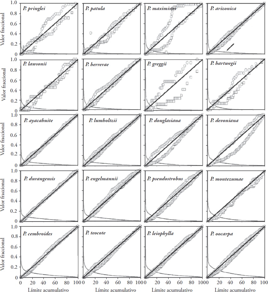
Figure 1 Analysis of the adjustment of the potential distribution models for 20 pine species in Mexico, using the ROC technique.
The analysis of the results shows that both, the AUC value and the relative probability value (RPV), significantly decrease (p≤0.001) as the number of species records increases (Figure 2A and 2B). Stockwell and Peterson (2002) showed that the modeling of any species depends on the quantity and quality of the data; of the latter, the geographic precision of its location suggest that, for the prediction to be robust, a minimum of 50 records should be used. Although species modeling with less than six records was published (Aguirre and Duivenvoorden, 2010), these are reported as non-significant. In our study, the records varied from 33 in P. greggii to 1,244 in P. cembroides (Figure 1), and it is clear that the modeling of the first species might not be robust due to having few records, and the rest of the species presents more than 60 data. It follows that the fit of the model increases with fewer registers, but underestimates and overestimates the predictions (Figure 2A). Elith et al. (2006) showed that parameter estimation in MaxEnt is critical when the sample size is small, and vice versa.
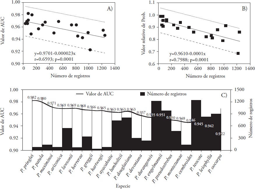
Figure 2 Relationship between values of the area under the curve, AUC (A), relative value of probability (B) and number of records. Trend of AUC values with respect to the number of records of each species (C).
The average value of the AUC of all the species was 0.959, with P. pringlei 0.982, P. patula 0.980 and P. maximinoi 0.971 as the species with the highest adjustment, contrary to that observed with P. oocarpa 0.922, P. leiophylla 0.942 and P. teocote 0.945 (Figure 2C). Even the latter value is very acceptable, since Phillips and Dudík (2008) established that the closer to 1 the value of the AUC is the better model. In addition, this average exceeds the value 0.75 suggested by Elith et al. (2006) and Aguirre and Duivenvoorden (2010), who assure that AUC values greater than 0.75 indicate that predictions based on only presence data are sufficiently precise to establish management plans.
The modeling of conifers potential distribution for this study using MaxEnt can be considered reliable. Aguirre and Duivenvoorden, (2010) reported an average AUC of 0.924, lower than the average of our study (0.959) but varying from 0.999 to 0.766. In P. pringlei, P. patula, P. maximinoi, P. teocote, P. leiophylla and P. oocarpa studied by these authors, the modeling of all of them improved in our study with AUC ranging from 0.928 to 0.967. With 391 records P. herrerae, Ávila et al. (2014) reported an AUC value of 0.973, similar to our study (Figure 1). These variations in model fit and prediction zones are due to the number of records used and their geographic location. In 11 modeled species by Ramos-Dorantes et al. (2017), and considered in our study, the average AUC was 0.966, slightly higher than that in our study (0.959). In 54.5 % of them, our research improved modeling: P. ayacahuite, P. greggii, P. hartwegii, P. patula, P. pseudostrobus and P. teocote. The model adjustment is not always good, in Pinus oocarpa Schiede ex Schltdl. the AUC value was only 0.548, and 0.445 in Abies guatemalensis Rehd. (Cruz-Cárdenas et al., 2016), but using other bioclimatic variables, a value close to 0.5 is really a random value (Felicísimo et al., 2012).
Environmental variables that model the distribution of the species
When considering the first three variables in each species model, the ones that contributed the most to predicting their distribution are altitude, Bio10 and Bio1, in 10, 9 and 6 species, respectively (Table 3). However, a single variable (Bio4) can explain 57.4 % of the potential distribution of P. lawsonii. The bioclimatic profile is different between species (Table 3) and depends on its geographical distribution in the country. In this regard, Eguiluz (1982) associated the distribution of 77 taxa of the Pinus genus throughout Mexico, and showed that several of them depend on: 1) maximum temperature, 11 species where recorded up to 45 °C, including P. pinceana, P. pseudostrobus var. Stevezii Mart., P. greggii and P. oocarpa; 2) minimum temperature, up to -23 °C, where P. ayacahuite, P. brachyptera, P. lumholtzii, P. engelmannii and Pinus arizonica grow; 3) precipitation, P. radiata var. binata Lem and P. greggii in 100 and 2900 mm of annual precipitation; 4) altitude, P. muricata D. Don and P. hartwegii Lind. grow between 120 to 4000 masl.
Table 3 Environmental variables with the highest contribution percentage in the prediction of pine potential distribution in Mexico and their bioclimatic profile.
| Especie | Var | % | Intervalo | Var | % | Intervalo | Var | % | Intervalo |
| Ppr | Bio4 | 57.4 | 1974 - 669 | Altitud | 27.1 | 2959 - 885 | Bio7 | 4.5 | 23.7 - 15.9 |
| Ppa | Bio10 | 36.5 | 24.2 - 11.0 | Bio7 | 13.3 | 23.8 - 15.7 | Bio5 | 12.3 | 31.8 - 19.3 |
| Pma | Bio4 | 33.1 | 2878 - 437 | Bio12 | 28.2 | 2870 - 761 | Altitud | 20.9 | 3001 - 428 |
| Par | Bio1 | 45.8 | 20.3 - 9.5 | Altitud | 14.4 | 3079 - 1051 | Bio11 | 9.9 | 15.3 - 2.5 |
| Pla | Bio4 | 46.4 | 2850 - 505 | Altitud | 28.9 | 3052 - 124 | Pendiente | 14.2 | 18.52 - 1.282 |
| Phe | Bio18 | 16.5 | 828 - 95 | Bio10 | 15.8 | 25.4 - 14.4 | Altitud | 15.0 | 2882 - 1025 |
| Pgr | Altitud | 22.2 | 2870 - 181 | Pendiente | 19.4 | 16.05 - 0.852 | Bio2 | 11.8 | 16.2 - 11.3 |
| Pha | Bio10 | 40.3 | 25.7 - 8.1 | Altitud | 22.9 | 3902 - 790 | Bio12 | 11.1 | 2363 - 692 |
| Pay | Bio1 | 33.1 | 23.6 - 9.1 | Bio10 | 27.3 | 24.9 - 11.4 | Bio17 | 5.2 | 151 - 10 |
| Plu | Bio5 | 52.6 | 33.4 - 22.1 | Bio3 | 13.0 | 68 - 51 | Bio19 | 8.2 | 274 - 32 |
| Pdo | Bio10 | 21.4 | 25.3 - 12.1 | Bio13 | 15.2 | 431 - 128 | Bio16 | 9.8 | 1218 - 311 |
| Pde | Bio7 | 22.4 | 26.8 - 15.0 | Bio10 | 15.3 | 25.9 - 12.6 | Bio8 | 12.5 | 24.8 - 11.7 |
| Pdu | Bio1 | 42.4 | 21.6 - 9.8 | Altitud | 13.1 | 3079 - 921 | Bio18 | 10.6 | 788 - 165 |
| Pen | Bio1 | 24.9 | 23.2 - 10.1 | Bio11 | 16.9 | 19.3 - 2.8 | Bio18 | 15.4 | 788 - 125 |
| Pps | Bio5 | 33.0 | 33.6 - 15.9 | Bio10 | 20.7 | 25.5 - 8.4 | Bio12 | 18.0 | 3546 - 487 |
| Pmo | Bio4 | 20.6 | 5469 - 575 | Pendiente | 18.2 | 25.5 - 0.7 | Altitud | 16.8 | 3686 -664 |
| Pce | Bio1 | 37.0 | 20.1 - 10.3 | Altitud | 27.2 | 3132 - 1068 | Bio12 | 10.3 | 1253 - 191 |
| Pte | Bio5 | 45.3 | 33.9 - 17.5 | Bio10 | 11.1 | 26.7 - 9.7 | Bio8 | 7.5 | 26.2 - 8.7 |
| Ple | Bio1 | 35.1 | 23.4 - 9.9 | Bio10 | 28.8 | 25.1 - 11.7 | Bio18 | 11.7 | 793 - 125 |
| Poo | Bio16 | 29.3 | 1670 - 207 | Bio8 | 25.4 | 26.5 - 11.3 | Bio13 | 15.9 | 635 - 72 |
Var: bioclimatic and topographic variables; %: contribution percentage according to the Jackknife test. Ppr = P. pringlei; Ppa = P. patula; Pma = P. maximinoi; Par = Pinus arizonica; Pla = P. lawsonii; Phe = P. herrerae; Pgr = P. greggii; Pha = P. hartwegii; Pay = P. ayacahuite; Plu = P. lumholtzii; Pdo = P. douglasiana; Pde = P. devoniana; Pdu = P. durangensis; Pen = P. engelmannii; Pps = P. pseudostrobus; Pmo = P. montezumae; Pce = P. cembroides; Pte = P. teocote; Ple = P. leiophylla; Poo = P. oocarpa. Bio1, ..., Bio19 defined in Table 2.
The principal component analysis shows two clearly defined groups: a compact group of species (Pinus cembroides, P. durangensis, P. arizonica, P. lumholtzii, P. leiophylla, P. herrerae, P. leiophylla and P. ayacahuite) were especially distributed to Bio1, Bio11, Bio18 and Bio19; and a second group highlighting P. devoniana, P. douglasiana and P. oocarpa, depending on Bioclim variables derived from precipitation, Bio13, Bio15 and Bio16 (Figure 3A). Pinus greggii showed a different response to other species, and its distribution depends on the driest month's precipitation (Bio14) and exposure. When considering a greater than 10 % contribution, altitude appears in the model structures in more than 55 % of the species, followed by Bio10 (50 %) and Bio1 (35 %); the variables that do not explain more than that value are Bio6, Bio9, Bio15, Bio17, Bio19 and exposure (Figure 3B).
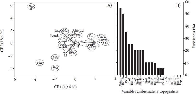
Figure 3 Principal component analysis of the modeling contribution of bioclimatic and topographic variables in 20 Mexican conifers species (A) and frequency in the models (B). The symbols are explained in Materials and Methods.
Similar to our study and derived from the Jackknife test, Téllez et al. (2005) reported that the variables that explain P. arizonica, P. devoniana, P. durangensis and P. pseudostrobus distribution are Bio1 and Bio12. In 12 conifers species evaluated by Ramos-Dorantes et al. (2017), Bio1 was the most important variable, 11 of these species included in this same study responding to this same bioclimatic variable. For Pinus herrerae Martínez, the maximum temperature and altitude (1985 - 2227 masl) determine its distribution (Ávila et al., 2014), as well as in our results, which does not explain conifer species distribution. Research by Cruz-Cárdenas et al. (2016) at a regional scale, on eight species included in our study, contrasts with our data: Bio6 explains 92.3 % of the distribution of P. douglasiana, 76.7 % of P. lawsonii, 92.4 of P. pseudostrobus and 92.3 % of P. teocote; and agree with P. montezumae (48.9 %), when observing that altitude determines its distribution.
Surface and potential distribution maps
The three species with the largest potential distribution area estimated by MaxEnt according to a probability greater than or equal to 0.70 are: P. montezumae, P. devoniana and P. pseudostrobus with 14,744.8, 14,436.1 and 11,594.8 km2 (Figures 4 and 5O, L and Ñ), while those with the smaller potential area were P. durangensis, P. lumholtzii and P. engelmannii with 0.1, 275.9 and 819.1 km2 (Figures 4 and 5N, J and M). Oaxaca (+) and Durango (*) are the states that register ideal area for nine species (Figure 4), Chihuahua for seven, Guerrero six, Michoacán and Puebla five (Figure 4), whereas seven states record conditions only for one species, each different. Of the registered species 50 % has a probability value greater than 0.9 (Figures 5A, B, C, E, F, G, H, L, O and S), and only P. durangensis does not have a surface within this range (Figure 5M).

Figure 4 Estimated area by species in a probability threshold greater than 0.70 and the three states of the country with highest conditions for the suitability of each species.
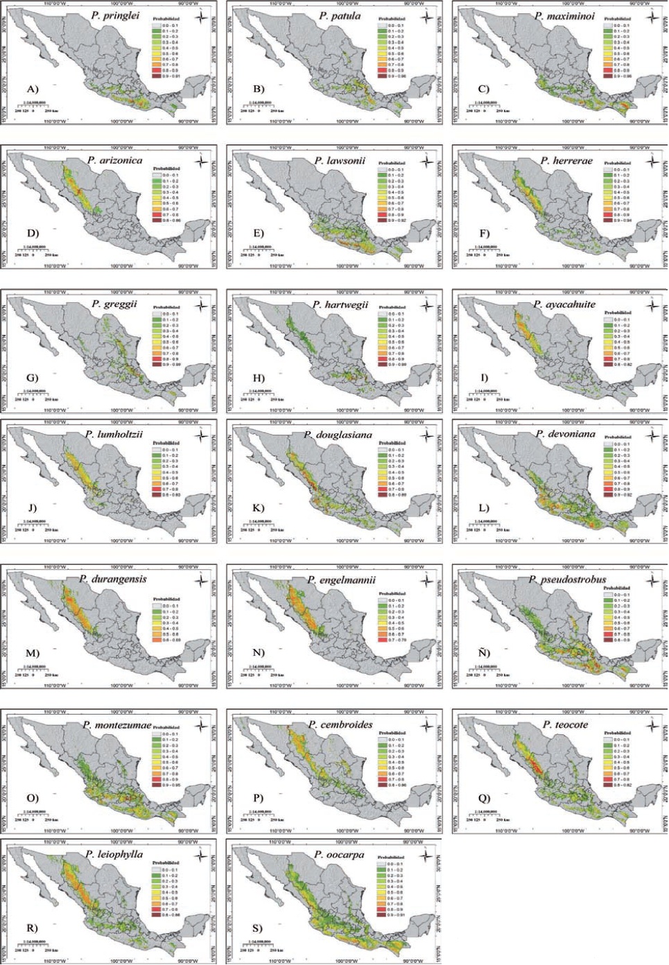
The comparison of the potential distribution areas of coniferous species in Mexico, between studies, would be ambiguous because they may represent different scales of information and spatial analysis (Ávila et al., 2014; Cruz-Cárdenas et al., 2016; Ramos-Dorantes et al., 2017). Besides, Téllez et al. (2005) and Aguirre and Duivenvoorden (2010) report distribution areas at the species and taxa level without indicating records number, and present areas in different probability ranges. Of these latter authors, the bioclimatic profile and geographic distribution is similar to that found here for P. arizonica, P. devoniana, P. durangensis and P. pseudostrobus. Stockwell and Peterson (2002) agree that the number of records is relevant in the quality of the prediction models and, therefore, the estimation of distribution areas is important, since Cruz-Cárdenas et al. (2016) indicate that species such as P. leiophylla and P. teocote under different climate change scenarios will reduce their distribution area. The delineation of the geographical distribution of the species studied here perfectly includes the five geographic zones reported by Sánchez-González (2008), and are useful in the assessment of the species distribution due to the effects of climate change (Phillips and Dudík, 2008).
Conclusions
The generated models can be considered reliable, since their AUC values were higher than 0.90. The delineation of the potential distribution of twenty species of conifers in Mexico has been updated, at different probability levels. The variables that make up the models are especially those derived from maximum temperature, altitude and precipitation; however, each species has specific bioclimatic requirements. Oaxaca and Durango have the ideal environmental characteristics to support the growth for nine conifers species. The bioclimatic profile determined for each species is relevant to establish management plans and increase their productive potential. Our proposed hypothesis is accepted because the bioclimatic variables adequately predict the potential distribution of the species studied.
Literatura Citada
Aguirre, G. J., and J. F. Duivenvoorden. 2010. Can we expect to protect threatened species in protected areas? A case study of the genus Pinus in México. Rev. Mex. Biodiv. 81: 875-882. [ Links ]
Ávila C., R., R. Villavicencio G., y J. A. Ruiz C. 2014. Distribución potencial de Pinus herrerae Martínez en el occidente del estado de Jalisco. Rev. Mex. Ciencias For. 5: 92-109. [ Links ]
Benito de Pando, B., y J. Peñas de Giles. 2007. Aplicación de modelos de distribución de especies a la conservación de la biodiversidad en el sureste de la Península Ibérica. GeoFocus. Rev. Int. Ciencia y Tecnol. Infor. Geogr. 7: 100-119. [ Links ]
Bradley, B., and E. Fleishman. 2008. Can remote sensing of land cover improve species distribution modelling. J. Biogeograp. 35: 1158-1159. [ Links ]
Cruz-Cárdenas, G., L. López-Mata L., J. T. Silva, N. Bernal-Santana, F. Estrada-Godoy, and J. A. López-Sandoval. 2016. Potential distribution model of Pinaceae species under climate change scenarios in Michoacán. Rev. Chapingo Serie Ciencias For. Ambiente 22: 135-148. [ Links ]
Dawson, B., and M. Spannagle. 2009. The Complete Guide to Climate Change. Routledge, New York. 436 p. [ Links ]
Eguiluz, P., T. 1982. Clima y distribución del genero Pinus en México. Rev. Ciencia For. 38: 30-44. [ Links ]
Elith, J., C Graham, R. Anderson, M. Dudík, S. Ferrier, A. Guisan, R. Hijmans, F. Huettmann, J. Leathwick, A. Lehmann, Li Jin, L. Lohmann G., B. Loiselle A., G. Manion, C. Moritz, M. Nakamura, Y. Nakazawa, McC. Overton J., A. Peterson T., S. Phillips J., K. Richardson, R. Scachetti-Pereira, R. Schapire E., J. Soberón, S. Williams, M. Wisz S., and N. Zimmermann E. 2006. Novel methods improve prediction of species distributions from occurrence data. Ecography 29: 129-151. [ Links ]
Felicísimo, A. M., J. Muñoz, R., Mateo R., y C. Villalba. 2012. Vulnerabilidad de la flora y vegetación españolas ante el cambio climático. Rev. Ecosist. 21: 1-6. [ Links ]
García, E. 1998. Comisión Nacional para el Conocimiento y Uso de la Biodiversidad (CONABIO). Climas, Clasificación de Köeppen, modificado por García. Carta de Climas, escala 1:1 000 000. México. [ Links ]
González, C., O. Wang, S. Strutz E., C. González S., V. Sánchez C., and S Sarkar. 2010. Climate change and risk of leishmaniasis in North America: predictions from ecological niche models of vector and reservoir species. Plos Neglected Trop. Dis. 4: 585 p. [ Links ]
Guisan, A., and N. E. Zimmermann. 2000. Predictive habitat distribution models in ecology. Ecol. Model. 135: 147-186. [ Links ]
Hijmans, J. R., S. Cameron E., J. L. Parra, P. G. Jones, and A. Jarvis. 2005. Very high resolution interpolated climate surfaces for global land areas. Int. J. Climatol. 25: 1965-1978. [ Links ]
INEGI. 2009. Aspectos generales del territorio mexicano. http://www.inegi.org.mx/inegi. [ Links ]
Kumar, S., and T. J. Stohlgren. 2009. MaxEnt modeling for predicting suitable habitat for threatened and endangered tree Canacomyrica monticola in New Caledonia. J. Ecol. Nat. Environ. 1: 094-098. [ Links ]
Morales, N. S. 2012. Modelos de distribución de especies: Software MaxEnt y sus aplicaciones en Conservación. Rev. Conserv. Amb. 2: 1-5. [ Links ]
Parmesan, C. 2006. Ecological and evolutionary responses to recent climate change. Ann. Rev. Ecol. Evol. Syst. 37: 637-669. [ Links ]
Peterson, A. T., V. Sánchez-Cordero, E. Martínez-Meyer, and A. Navarro-Sigüenza. 2006. Tracking population extirpations via melding ecological niche modeling with land-cover information. Ecol. Model. 195: 229-236. [ Links ]
Phillips, S. J., and M. Dudik. 2008. Modeling of species distributions with Maxent: new extensions and a comprehensive evaluation. Ecography 31: 161-175. [ Links ]
Phillips, S. J., R. P. Anderson, and R. E. Schapire. 2006. Maximum entropy modeling of species geographic distributions. Ecol. Model. 190: 231-259. [ Links ]
Ramírez-Herrera C., J. J. Vargas-Hernández, y J. López-Upton. 2005. Distribución y conservación de las poblaciones naturales de Pinus greggii. Acta Bot. Mex. 72: 1-16. [ Links ]
Ramos-Dorantes, D. B., J. L. Villaseñor, E. Ortiz, and D. S. Gernandt. 2017. Biodiversity, distribution, and conservation status of Pinaceae in Puebla, Mexico. Rev. Mex. Biodiv. 88: 215-223. [ Links ]
Sánchez-González, A. 2008. Una visión actual de la diversidad y distribución de los pinos de México. Madera y Bosques 14: 107-120. [ Links ]
Stockwell, R. B. D., and A. Peterson T. 2002. Effects of sample size on accuracy of species distribution models. Ecol. Model. 148: 1-13. [ Links ]
Téllez, V. O., Y. M. Chávez H. A. Gómez Tagle Ch., y M. V. Gutiérrez G. 2005. Modelado bioclimático como herramienta para el manejo forestal: Estudio de cuatro especies de Pinus. Rev. Ciencia For. Méx. 29: 61-82. [ Links ]
Walther, G. R. 2010. Community and ecosystem responses to recent climate change. Philos. Trans. R. Soc. Lond. B. Biol. Sci. 365: 2019-2024. [ Links ]
Woodward, F. I. 1987. Climate and Plant Distribution. Cambridge University Press, Cambridge. UK. 177 p. [ Links ]
Yeaton, R. I. 1982. The altitudinal distribution of the genus Pinus in the western United States and Mexico. Bol. Soc. Bot. Méx. 42: 55-71. [ Links ]
Received: June 2017; Accepted: November 2017
 Este es un artículo publicado en acceso abierto bajo una licencia Creative Commons
