


Serviços Personalizados
Journal
Artigo
 texto em
  Inglês (pdf)
 Artigo em XML
 Referências do artigo
 Enviar este artigo por email
Indicadores
-
 Citado por SciELO
 -
 Acessos
Links relacionados
-
 Similares em
SciELO
Similares em
SciELO
Compartilhar

 Permalink
Agrociencia
versão On-line ISSN 2521-9766versão impressa ISSN 1405-3195
Agrociencia vol.52 no.7 Texcoco Out./Nov. 2018
Natural Renewable Resources
Taper functions for Eucalyptus urophylla clones established in commercial plantations in Huimanguillo, Tabasco, Mexico
1 Forestal. Campus Montecillo. Colegio de Postgraduados. Montecillo, Estado de México (forestjonathanhdez@gmail.com).
2 Instituto Nacional de Investigaciones Forestales, Agrícolas y Pecuarias (INIFAP). Campo experimental San Martinito, Tlahuapan, Puebla, México. 74060. (tamarit.juan@inifap.gob.mx).
3 United States Department of Agriculture Forest, Service. Techniques Analyst, 507 25th Street, Ogden, Utah, United States. (apeduzzi@fs.fed.us).
Taper functions allow modelling stem profile, estimating the dimensions of tree sections and the timber-yielding volume per type of products, and planning forest supply. The objective of this study was to develop a function that allows modelling the stem profile of Eucalyptus urophylla S. T. Blake clone trees established with commercial purposes in Huimanguillo, Tabasco, Mexico. With 2,133 pairs of data from 93 trees, ten taper models were fitted with the maximum likelihood method. The best model was selected according to the lowest values of the root mean square error (RMSE), the coefficient of variation, the bias and the highest adjusted coefficient of determination (R2 aj.). The fifth-degree polynomial model was the best statistically to model the stem profile of E. urophylla clones, because it includes the relative proportion of the height in each section of the total height. Autocorrelation was corrected by including in the fiiting a CAR(1) type autocorrelation structure. The polynomial model estimates in a reliable way the diameter and the height in clone trees from commercial plantations of E. urophylla.
Key words: Log profile; commercial volumen; eucalyptus clones; forest exploitation; Eucalyptus urophylla
Las funciones de ahusamiento permiten modelar el perfil fustal, estimar las dimensiones de las secciones del árbol y el volumen maderable por tipo de productos, así como planear el abastecimiento forestal. El objetivo de este estudio fue desarrollar una función que permitiera modelar el perfil fustal de árboles clonales de Eucalyptus urophylla S. T. Blake establecidos con fines comerciales en Huimanguillo, Tabasco, México. Con 2,133 pares de datos de 93 árboles se ajustaron diez modelos de ahusamiento con el método de máxima verosimilitud. El mejor modelo se seleccionó de acuerdo con los valores menores de la raiz del cuadrado medio del error (RCME), el coeficiente de variación, el sesgo y el mayor coeficiente de determinación ajustado (R2aj.); el modelo polinomial de quinto orden fue el mejor estadísticamente para modelar el perfil fustal de clones de E. urophylla, porque incluye la proporción relativa de la altura en cada sección en la altura total. La autocorrelación se corrigió al incluir en el ajuste una estructura de autocorrelación de tipo CAR(1). El modelo polinomial estima de forma confiable el diámetro y la altura en árboles clonales provenientes de plantaciones comerciales de E. urophylla.
Palabras clave: Perfil fustal; volumen comercial; clones de eucalipto; aprovechamiento forestal; Eucalyptus urophylla
Introduction
In the world, there are 264 million ha of forest plantations with 25 % made up of introduced species (FAO, 2010). Mexico occupied, until 2015, the fifth place in America with forests established through plantation or sowing, or both, in the process of forestation or reforestation (INEGI, 2014); among these, the use of species of fast growth stands out (Overbeerk et al., 2012). Eucalyptus is the second most used genus in the country to establish commercial forestry plantations (CFP) (SEMARNAT-CONAFOR, 2014) with around 32,452 ha planted (CONAFOR, 2015), and E. urophylla is the most frequently planted species in tropical climates (CONAFOR, 2012).
Estimating the volume and the distribution of timber-yielding products from natural forests and plantations is a need in forest management. The equations that describe stem profile or the taper functions are a feasible option for the accurate calculation of the dimensions and volumes of any part of the bole (Maldonado-Ayala and Návar, 2000; Cancino, 2006), or the distribution of products (Barrero et al., 2013). In addition, they are an essential component in the yield systems and in the sawtimber simulation (Gezan et al., 2009).
These functions describe the rate of diameter decrease in any part of the bole as it approaches the total height of the tree (Prodan et al., 1997; Torres and Magaña, 2001) and they vary according to the species, age, tree size, factors associated to management, and conditions of the site or density (Cancino, 2006). It is also possible to assess the influence of these factors on production (Barrero et al., 2013) and to suggest activities for technical management that modify the shape of the tree to attain the objectives set out through forest management (Sterba, 1980).
Due to the difficulty in describing the profile of a tree, models were based on biological principles (Rodríguez-Toro et al., 2016); some were based on the shape of regular geometrical bodies and others were built based on experimentation in function of the measurements that refer to each individual, without taking into account that they are related to a geometrical body (empirical), although this does not mean that one is better than the other (Cancino, 2006). The models can be polynomic, trigonometric, variable exponent, segmented or compatible with functions of total volume (Gezan et al., 2009). Some of the fitting techniques used are systems of seemingly unrelated equations (SUR) through root mean square error (RMSE) and full information maximum likelihood (FIML), because they make the estimators of the parameters consistent and asymptotically efficient, situation that does not happen with the method of ordinary least squares (OLS), which ignores the errors in the diameter along the stem. The greatest difficulty in estimating any of these is in the base and the tip of the tree (Cancino, 2006), which is why Cruz-Cobos et al. (2008) modelled this type of informaiton with the approach of mixed effects.
The bole shape, distribution of products, and yield of the trees should be understood in order to plan the harvesting activities of timber-yielding resources; in addition, Eucalyptus is a fast-growth species and the equations used must be in constant updating. Therefore, the hypothesis of this study was that the total and commercial volumes have a close relationship with the shape of the tree, and the objective was to develop a taper function that allows modelling the stem profile of clone trees of E. urophylla S. T. Blake established with commercial purposes in Huimanguillo, Tabasco, Mexico.
Materials and Methods
This study was performed with data obtained in plots with commercial forest plantations of clones of E. urophylla, one to seven years old, established in the municipality of Huimanguillo, Tabasco, Mexico. The local climate is warm humid (Am), with annual mean temperature of 26 °C and mean annual precipitation of 2,500 mm. The predominant soil unit is Feozem type (INEGI, 2005).
The sample consisted of 93 felled trees, from which 2,133 pairs of data were obtained along the stem. In each tree selected for its dominance within the stand, the diameter with bark (d) and the height (hm) were measured in sections 1 m long, beginning with the stump diameter (dt) and height (ht) until reaching the total height (H); the normal diameter (dn) was also included.
The taper models fitted to the set of data were selected from the international literature for their successful use in other studies (Table 1). The fitting of the models was carried out with the MODEL procedure of the SAS 9.2 software (SAS institute Inc., 2008) and the full information maximum likelihood (FIML) method. The evaluation and selection of the best model was carried out based on the highest value of the adjusted coefficient of determination by the number of parameters (R2aj.) and the lowest values in the Residual Sum of Squares (RSS), Root Mean Square Error (RMCE), the Coefficient of Variation (CV) and the Bias (E).
Table 1 Taper models (d) fitted to model stem profile of E. urophylla trees from CFP in Tabasco, Mexico.
| No. | Modelo | Expresión | Donde |
| (1) | Demaerchalk |
|
X = (H-hm)/H |
| (2) | Kozak |
|
X = (H-hm)/H |
| (3) | Forslund |
|
X = hm/H |
| (4) | Clutter |
|
__ |
| (5) | Cielito 1 |
|
X = (H-hm)/H |
| (6) | Cielito 2 |
|
X = hm/H |
| (7) | Cielito 3 |
|
X = (H-hm)/H |
| (8) | Polinomial |
|
X = hm/H |
| (9) | Newnham |
|
X = (H-hm)/(H-1.3) |
| (10) | Rustagi y Loveless |
|
X = (H-hm)/(H-1.3) |
dn: Normal diameter. H: Total height. hm: Height at different diameters along the stem.:(’ Parameters to be estimated.
A hierarchical criterion was used to ease the selection of the best model, for which the goodness of fit statistics was integrated (SCE, RCME, R2aj. , CV and E) and scored (Sakici et al., 2008), by assigning consecutive values from 1 to 10 in function of their value for each one of the statistics used, with 1 being the highest index and 10 the lowest. For example, a value of 1 is assigned to the model with least value in the RCME, while the next ones in ascending order will be scored with 2, 3, 4…10, as corresponds; this procedure is applied for SCE, CV and E. For R2aj., it is inverse and the value 1 is assigned to the model with highest value in this statistic. Then, for each model, the grading values of the statistics were added to obtain a total and the model with the lowest score was selected as the best.
The autocorrelation of the errors in the models was examined with the Durbin-Watson test (Augusto et al., 2009). To correct the autocorrelation problems of the taper model selected, an autorregresive model in continuous order (CAR(X)) was applied (Lara, 2011). The fitting was carried out with the structure (Zimmerman & Nuñez-Antón, 2001):
where Yij is the vector of the dependent variable, Xij the matrix of independent variables, B is the vector of the parameters to be estimated, eij is the j-th residue of the tree i, Ik = 1 for j>k and is 0 for j≤k, pk is the autorregresive parameter of order k to be estimated, hij -hij-k is the distance that separates the height of the j-th measurement of the height of measurement j-th-k in each tree (hij >h ij-k ) and ε ij is the random error (Álvarez et al., 2005; Barrios et al., 2014).
The number of lags applied in the model CAR(X) was defined after evaluating the Durbin-Watson statistic (DW) which is defined in a value that was higher than 1.5 and close to 2 (Verbeek, 2004). In an analogous way, the residuals were analyzed graphically to verify problems of heterocedasticity, which according to Kozak (1997), are the most important disadvantages in this type of studies and violate the assumptions of the regression.
The total volume was estimated with the taper equation selected, by integrating the diameter d along the stem in relation to hm as a solid in revolution using the following expression:
where
The taper model chosen was used to estimate hm at any commercial diameter of interest, after solving for the variable of the mathematical expression used.
Results and Discussion
All the values from the parameters corresponding to each fitted model were significant with a 95 % statistical confidence and the approximate standard error was small in its majority, with the exception only of parameter β 2 from the Demaerchalk (1) model, which was very large (Table 2). The statistics of fit in the ten taper models and the final score of the system used indicate that the models Cielito 3 (7) and Fifth degree polynomial (8) are the most statistically stable (Table 3).
Table 2 Values of the parameters of the taper models for clone trees of E. urophylla in Huimanguillo, Tabasco, Mexico.
| Modelo | Parámetros | Estimación | Error estándar aproximado | Valor de t | Pr > |t| |
| (1) | β 1 | 0.3345 | 0.0090 | 37.22 | <0.0001 |
| β 2 | 44.1618 | 3.9580 | 11.16 | <0.0001 | |
| β 3 | 0.0001 | 0.0000 | 192.31 | <0.0001 | |
| β 4 | 1.4947 | 0.0156 | 95.71 | <0.0001 | |
| (2) | β 1 | -2.1846 | 0.0040 | -550.50 | <0.0001 |
| β 2 | 1.0005 | 0.0015 | 688.04 | <0.0001 | |
| (3) | β 1 | 0.9682 | 0.0234 | 41.35 | <0.0001 |
| β 2 | 1.3249 | 0.0291 | 45.61 | <0.0001 | |
| (4) | β 1 | 0.3870 | 0.0300 | 12.90 | <0.0001 |
| β 2 | 0.6696 | 0.0150 | 44.74 | <0.0001 | |
| β 3 | 0.8105 | 0.0089 | 91.45 | <0.0001 | |
| β 4 | -0.6593 | 0.0198 | -33.36 | <0.0001 | |
| (5) | β 1 | 0.6171 | 0.0313 | 19.74 | <0.0001 |
| β 2 | -0.6144 | 0.0968 | -6.35 | <0.0001 | |
| β 3 | 1.2550 | 0.0712 | 17.62 | <0.0001 | |
| (6) | β 1 | 1.4268 | 0.0067 | 214.61 | <0.0001 |
| β 2 | -6.2136 | 0.0948 | -65.57 | <0.0001 | |
| β 3 | 14.7676 | 0.3654 | 40.41 | <0.0001 | |
| β 4 | -16.6882 | 0.5047 | -33.06 | <0.0001 | |
| β 5 | 6.7078 | 0.2289 | 29.30 | <0.0001 | |
| (7) | β 1 | 0.6916 | 0.0053 | 131.31 | <0.0001 |
| β 2 | 0.9627 | 0.0105 | 91.51 | <0.0001 | |
| β 3 | 15.7811 | 0.5157 | 30.60 | <0.0001 | |
| (8) | β 1 | 1.2729 | 0.0030 | 431.75 | <0.0001 |
| β 2 | -5.5526 | 0.1032 | -53.83 | <0.0001 | |
| β 3 | 4.8763 | 0.0832 | 58.60 | <0.0001 | |
| β 4 | -3.7086 | 0.0575 | -64.54 | <0.0001 | |
| β 5 | -2.6549 | 0.0386 | -68.75 | <0.0001 | |
| β 6 | -1.7863 | 0.0244 | -73.17 | <0.0001 | |
| (9) | β 1 | 1.0099 | 0.0022 | 451.58 | <0.0001 |
| β 2 | 0.8179 | 0.0091 | 89.95 | <0.0001 | |
| (10) | β 1 | 0.0198 | 0.0012 | 17.05 | <0.0001 |
| β 2 | 0.9263 | 0.0051 | 180.90 | <0.0001 | |
| β 3 | 1.0048 | 0.0141 | 71.27 | <0.0001 |
Table 3 Goodness of fit statistics for the taper models evaluated for clone trees of E. urophylla in Huimanguillo, Tabasco, Mexico.
| Modelo | SCE | RCME | R2aj. | CV | E | Cal. total |
| (1) | 0.628 | 0.0172 | 0.938 | 15.15 | 0.0015 | 17 |
| (2) | 0.797 | 0.0193 | 0.922 | 17.13 | 0.0028 | 34 |
| (3) | 0.977 | 0.0214 | 0.901 | 18.62 | 0.0048 | 40 |
| (4) | 0.663 | 0.0177 | 0.935 | 15.51 | 0.0004 | 18 |
| (5) | 0.699 | 0.0181 | 0.932 | 15.87 | 0.0015 | 23 |
| (6) | 0.539 | 0.0159 | 0.947 | 13.88 | 0.0022 | 12 |
| (7) | 0.544 | 0.016 | 0.947 | 14.12 | 0.0003 | 11 |
| (8) | 0.449 | 0.0145 | 0.956 | 12.89 | 0.0017 | 9 |
| (9) | 0.787 | 0.0196 | 0.913 | 16.18 | 0.0027 | 34 |
| (10) | 0.689 | 0.0184 | 0.924 | 15.55 | 0.0003 | 22 |
SCE: Residual Sum of Squares. RCME: Root Mean Square Error. R2aj. : Coefficient of determination adjusted by the number of parameters. CV: Coefficient of Variation. E: Bias. Cal. total: Total score of the statistics.
The models Cielito 3 (7) and Fifth degree polynomial (8) were the best when applying the criteria proposed by Trincado and Leal (2006) and Augusto et al. (2009), according to the values of R2aj. , RCME and CV, in addition to the scoring system used by Sakici et al. (2008) and implemented by Tamarit et al. (2014). The statistical fit is similar to what was found for teak plantations by Lara (2011), who also defined that a polynomial model was better to describe the stem profile from the numerous inflection points that it can describe.
The differences between the data observed and the estimation of models Cielito 3 and Fifth degree polynomial were lower than 15 %, which is an acceptable percentage in these studies according to Turribuano and Salinas (1998), who used taper functions with Pseudotsiga mensiensii in Chile; the differences happen primarily close to the dimensions of dn and dt. In addition, the values agree with those reported by Gezan et al. (2009) when using the simple models by Bruce et al. (1968) and Kozak (1988), which fitted adequately to the population evaluated. Kozak et al. (1969) and Kozak (1997) indicate that this type of simple models present biases primarily in the basal part of the tree and in the estimation of the final diameter to converge to zero. However, in studies with taper models of segmented type or fitted under the approach of mixed effects, this type of errors was reduced.
The value of the DW test for the ten functions used varied between 1.15 and 0.54, which shows that in every case there is presence of autocorrelation of the errors (Institute Inc. Statistical Analysis System, 2008). The models Cielito 3 and Fifth degree polynomial, which had the best value from the scoring and fitting system, were corrected for the autocorrelation problem by applying a lag in the residuals (lar1) with the structure CAR(1). The values of goodness of fit are adequate and the parameters of the final models proposed are significant and, in addition, the correction generated values in the DW statistic of 1.82 and 1.75, respectively, which indicates that the problem was corrected (Table 4).
Table 4 Statistics of goodness of fit and values of the parameters from the taper models Cielito 3 and Fifth degree polynomial corrected by autocorrelation for trees of E. urophylla in Huimanguillo, Tabasco, Mexico.
| Modelo | SCE | RCME | R2aj. | DW | Parámetros | Estimación | EEA | Valor de t | Pr > |t| |
| 7 | 0.374 | 0.0133 | 0.963 | 1.75 | β 1 | 0.6953 | 0.00802 | 86.66 | <0.0001 |
| β 2 | 1.0812 | 0.01070 | 100.92 | <0.0001 | |||||
| β 3 | 17.4023 | 0.05832 | 29.84 | <0.0001 | |||||
| 8 | 0.332 | 0.0125 | 0.967 | 1.82 | β 1 | 1.3130 | 0.00256 | 512.10 | <0.0001 |
| β 2 | -6.0812 | 0.01219 | -49.87 | <0.0001 | |||||
| β 3 | 5.1035 | 0.09890 | 51.59 | <0.0001 | |||||
| β 4 | -3.8067 | 0.06900 | -55.16 | <0.0001 | |||||
| β 5 | -2.6987 | 0.04660 | -57.91 | <0.0001 | |||||
| β6 | -1.8051 | 0.02950 | -61.18 | <0.0001 |
SCE: Residual Sum of Squares. RCME: Root Mean Square Error. R2aj. : Coefficient of determination adjusted by the number of parameters. DW: Durbin-Watson test. EEA: Approximate standard error.
The graphic behavior of the estimated tapering with the models selected is similar to that reported by Pompa et al. (2009), Pompa-García et al. (2009) and Tapia and Návar (2011), since the trend of decreasing diameter (d) is observed as the height (hm) approaches the total height (H) of the log, which is why both models are adequate to describe the tree profile of this species in the plots studied (Figure 1).
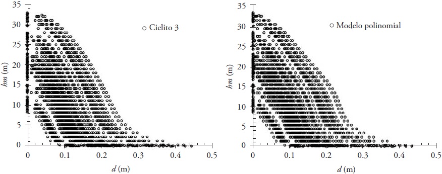
Figure 1 Prediction of the tree profile of E. urophylla clones with the models Cielito 3 and Fifth degree polynomial in Huimanguillo, Tabasco, Mexico.
The comparative of values of observed diameter versus predicted diameter shows their similarity (Figure 2) and the trend is consistent with that found in high values of d by Lara (2011) when analyzing five taper models.
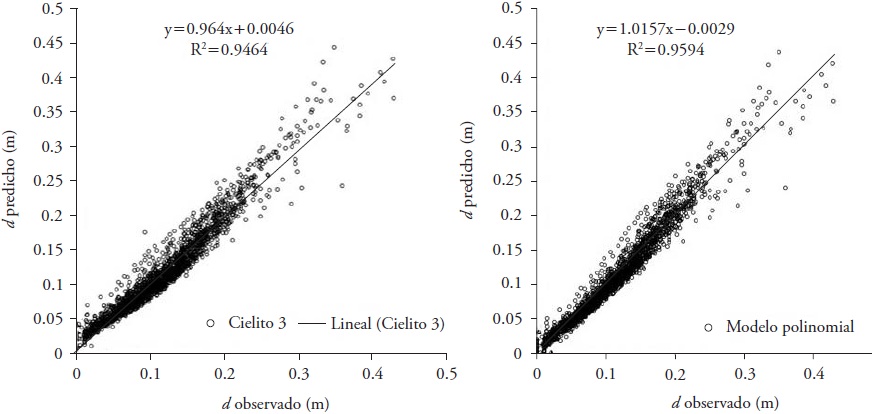
Figure 2 Observed diameter vs predicted diameter of the taper models Cielito 3 and Fifth degree polynomial fitted for clone trees of E. urophylla in Huimanguillo, Tabasco, Mexico.
The graphic analysis of the residuals of the models Fifth degree polynomial and Cielito 3 does not indicate problems of heterocedasticity (Figure 3), result that agrees with that reported by Fassola et al. (2007) when analyzing the taper model of Bi in E. grandis and Lara (2011) for Tectona grandis with the models by Forslund, González, Kozak, Ormerod and Fifth degree polynomial.
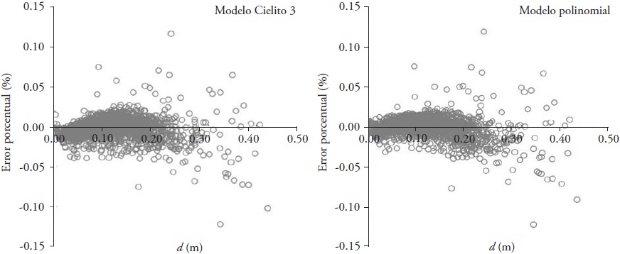
Figure 3 Residuals of the taper models selected for clone trees of E. urophylla in Huimanguillo, Tabasco, Mexico.
When verifying the percentage errors of the estimation of tapering at different heights of the stem in the corrected models, it is observed that the deviation of the estimates in the two models selected is lower than 12 % in the tree section from the base to the normal diameter; in the rest, the errors in the predictions are lower than 2 % (Figure 4). The distribution of the percentage errors throughout the stem takes place in a similar manner to that reported by Fassola et al. (2007), where the highest proportion was found in the lower parts of the height of the normal diameter.
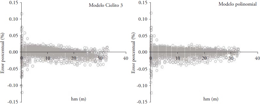
Figure 4 Percentage error of estimation of d at different hm in the stem through the models Cielito 3 and Fifth degree polynomial, fitted for clone trees of E. urophylla in Huimanguillo, Tabasco, Mexico.
When considering the lowest values in SCE, RCME and CV, the highest statistics of R2aj. and DW, in addition to not having apparent problems of heterocedasticity and deviations in the estimation, the Fifth degree polynomial model (model 8, Table 1) was selected as the best for the description of the stem profile of clone trees of E. urophylla under plantation conditions.
The model selected is reliable in the description of the tree profile. Lara (2011) and Orfanó et al. (2006) found good results for teak in Brazil when using various types of polynomial models, while in Argentina, Fassola et al. (2007) and Crechi et al. (2008) obtained good fits for E. grandis and Grevillea robusta, respectively.
To estimate the commercial height at any diameter of interest of the stem with the model proposed, the equation that estimates hm presents in its solution imaginary roots that can be reduced algebraically until being eliminated. Therefore, the solution was obtained in two ways. The first was by implementing in the SOLVER tool of the Excel Microsoft package, a numerical approximation for heights at different sections, where d = dc , in which the value of hm is changing and gives the solution, and the expression used is the following:
where dn is the normal diameter, Xi is an approximation of SOLVER to zero and dc represents the commercial diameter established.
The second way is proposed by Cruz-Cobos et al. (2008), and consists in using the iterative method suggesting a partial and redundant solution in X. The approximation to the value sought is the product of the multiplication of the value of such a partial solution (Xj) and the total height (H), with which this partial value is defined when the absolute difference estimated between a previous solution and the one used is either constant or the least possible, after the realization of the necessary iterations. The expression for this model is the following:
where Xj is the iterative approximation and partial solution for hm.
When verifying in the two procedures the convergence when d = dn, it was obtained that hm is equal to the height of 1.3 m and with regards to H the average deviation is lower than 1 %, situation that is desirable to estimate the height at any diameter established or to calculate the Vc with the dimensions given.
In order to determine the change of dendrometric shape of the stem in percentage in relation to the total height, the values estimated from the parameters and the second derivate
To complement the description of the tree profile and to perform accurate estimations of
commercial volume at different heights of the stem or to determine the
distribution of products, the Vc model compatible with the
taper function was obtained (15). This model is the result of the mathematical
integration of the fifth degree polynomial model in relation to
hm, defining the limits between the total height and the
stump height (hm=0) of expression (12):
Once this function is integrated and evaluated between 0 and hm, with later simplification, we find that the equation of commercial volume (Vc) at any height hm on the stem was:
When using this expression of commercial volume, although defining the value of hm as H, the total volume model is obtained of the shape:
The model can be defined as a model of constant shape
By substituting the parameters estimated of the taper model (8), a model of constant shape factor was obtained where
The fitting of the commercial volume equation resulting from the integration of the fifth degree polynomial model, on its own, tends to present non-significant parameters. However, the inclusion in a simultaneous system of the expressions (8) and (16) does not present this inconvenient because the colinearity between its parameters is broken. This allows estimating in a reliable way the comercial volumen at a given diameter or height; the expression coincides with what was obtained by Orfanó et al. (2006) and Lara (2011) for this model. By simultaneously fitting the compatible system of taper-commercial volumen using the technique of maximum likelihood, problems of autocorrelation and heterocedasticity are observed, which is why it was decided to add a lag (lar(1)) with a model of type CAR(X), both to d and to Vc in order to correct the problem, in addition to weighing the residuals of the latter to reduce the heterocedasticity problem. Diéguez-Aranda et al. (2009) point out that when estimating all the parameters of the system simultaneously, the residual sum of square errors is optimized. With this, the errors in the prediction are minimized, both of the diameter at different heights and of the volume. The values of the parameters are significant and the statistics of the simultaneous fit of the compatible system of taper and commercial volume are adequate (Table 5).
Table 5 Values of the statistics and parameters of simultaneous fit of tapering and commercial volume for E. urophylla in Huimanguillo, Tabasco, Mexico.
| Modelo | SCE | RCME | R2 ajustada | Parámetros | Estimación | EEA | Valor de t | Pr > |t| |
| d | 0.274 | 0.012 | 0.966 | β 1 | 1.0399 | 0.0047 | 221.85 | <0.0001 |
| Vc | 1.779 | 0.030 | 0.979 | β 2 | -1.1466 | 0.0304 | -37.70 | <0.0001 |
| β 3 | -0.2389 | 0.0384 | -6.23 | <0.0001 | ||||
| β 4 | 0.8769 | 0.0666 | 13.17 | <0.0001 | ||||
| β 5 | 0.6111 | 0.1145 | 5.34 | <0.0001 | ||||
| β 6 | -0.9743 | 0.0126 | -77.44 | <0.0001 | ||||
| lar(1) | 0.5823 | 0.0073 | 80.30 | <0.0001 |
SCE: Residual Sum of Squares. RCME: Root Mean Square Error. R2aj. : Coefficient of determination adjusted by the number of parameters. DW: Durbin-Watson test. EEA: Approximate standard error.
The statistics of fit both for d and Vc indicate a description of the data higher than 96 % and all the parameters are significant, which indicates a good statistical fit to the data used. In addition, and to correct the autocorrelation in d, the value of the DW test was equal to 1.83, which indicates the inexistence of these problems, according to Barrios et al. (2014), because the value approaches 2 in the Durbin-Watson test. However, in this type of fit the contrast between the variables observed and those predicted should be examined graphically.
Figure 5 (A and B) shows the trend of the estimations of accumulated volume (Vcacumulado) in relation to d and hm, which are similar to those reported by Tamarit et al. (2014) for estimation with the model of Vc . In addition, the data observed were compared against those predicted by the model (Figure 5C).
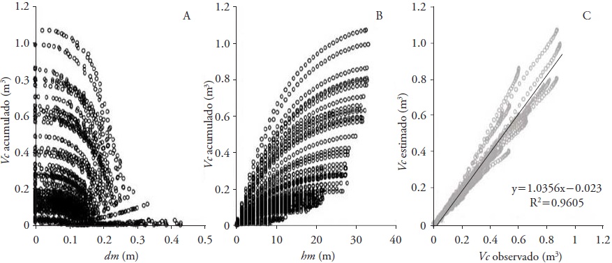
Figure 5 Behavior between d and hm in relation to the Vc (A and B) and graph of the data observed vs predicted from the model of Vc (C) for E. urophylla in Huimanguillo, Tabasco, Mexico.
The estimations of Vc with the function generated from the fifth degree polynomial model are good, since the average bias is only 4.41 %, although it can present the inconvenience of the bias increasing and the Vc being overestimated in trees with commercial volumes higher than 0.4 m3, which is why the range of applicability of the function is for individuals that have volume lower than the one mentioned.
The equation of variable form derived from the model (18) to estimate the total volume can be used in a reliable way. However, the compatible expression simultaneously fitted to calculate the commercial volume (16) has good statistical values, but it tends to present biases. In addition, to model the taper it is suggested to use the parameters obtained from the fitted fifth degree polynomial model or else to test in its fitting the inclusion of random effects that allow evaluating the effect of the variability of the genetic base and the changing profile of trees.
Conclusion
The function of the tree profile suggested can be used to describe the taper and to determine the height at any diameter established, which allows estimating the distribution of products or the commercial volume in trees from existing commercial forest plantations, due to the close relationship of the tree shape with the distribution of volume along the stem. However, because it is a fast-growing species under constant genetic improvement (clones), the continuous updating of this type of forestry tools is essential for more precise calculations in the time of establishement, growth and development of CFP with new clones, since the volume yield of individuals has a close relationship with the shape and size of the Eucalyptus urophylla trees.
Literatura Citada
Álvarez J. G., M. Barrio, F. Castedo-Dorado, U. Diéguez-Aranda, y A. D. Ruiz-González. 2005. Modelos para la gestión forestal: una revisión de las metodologías de construcción de modelos de masa. 5° Congreso Forestal Nacional, Portugal. 13 p. [ Links ]
Augusto, C. T., J. O. Vargas M., y M. Escalier H. 2009. Ajuste y selección de modelos de regresión para estimar el volumen total de árboles. Documento Técnico No. 5. Escuela de Ciencias Forestales de la Universidad Mayor de San Simón. Cochabamba, Bolivia. 27 p. [ Links ]
Barrios A., A. M. López, y V. Nieto. 2014. Predicción de volúmenes comerciales de Eucalyptus grandis a través de modelos de volumen total y de razón. Colombia For. 17: 137-149. [ Links ]
Barrero M., H., D. Álvarez-Lazo, e Y. Alonso-Torrens. 2013. Modelos del perfil de fuste para Pinus caribaea var. caribaea en la provincia Pinar del Río, Cuba. Rev. Científ. Avances 15: 259-268. [ Links ]
Bruce, D., R. Curtis, and G. Vancoevering. 1968. Development of a system of taper and volume tables for red alder. For. Sci. 14: 656-658. [ Links ]
Cancino C., J. O. 2006. Dendrometría básica. Universidad de Concepción. Facultad de Ciencias Forestales. Departamento de Manejo de Bosques y Medio Ambiente. http://repositorio.udec.cl/xmlui/handle/123456789/407 (Consulta: diciembre 2015). [ Links ]
CONAFOR (Comisión Nacional Forestal). 2012. Situación actual y perspectivas de las plantaciones forestales comerciales en México. México: Comisión Nacional Forestal. http://www.conafor.gob.mx/web/temas-forestales/plantaciones-forestales/ Consulta: diciembre 2015. [ Links ]
CONAFOR (Comisión Nacional Forestal). 2015. Plantaciones forestales comerciales. http://www.conafor.gob.mx/web/temas-forestales/plantaciones-forestales/ (Consulta: diciembre 2015). [ Links ]
Crechi, E., A. Keller, y H. Fassola. 2008. Desarrollo de una ecuación de forma-volumen relativo para la estimación de diferentes volúmenes de Grevillea robusta A. en Misiones, Argentina. XIII Jornadas Técnicas Forestales y Ambientales. Facultad de Ciencias Forestales, UNaM-EEA Montecarlo, INTA. Misiones, Argentina. 10 p. [ Links ]
Cruz-Cobos, F., H. M. De los Santos-Posadas, y J. R. Valdez-Lazalde. 2008. Sistema compatible de ahusamiento-volumen para Pinus cooperi Blanco en Durango, México. Agrociencia 42: 473-485. [ Links ]
Diéguez-Aranda, U., A. Alboreca R, F. Castedo-Dorado, J. G. Álvarez-González, M. Barrio-Anta, F. Crecente-Campo, J. M. González-González, C. Pérez-Cruzado, R. Rodríguez-Soalleiro, C. A. López-Sánchez, M. A. Balboa-Murias, J. J. Gorgoso-Varela, y F. Sánchez Rodríguez. 2009. Herramientas Selvícolas para la Gestión Forestal Sostenible en Galicia. Xunta de Galicia. Lugo, España. 259 p. [ Links ]
Gezan A. S., P. C. Moreno M., y A. Ortega. 2009. Modelos fustales para renovales de roble, raulí y coigüe en Chile. Bosque 30: 61-69. [ Links ]
FAO (Organización de las Naciones Unidas para la Agricultura y la Alimentación). 2010. Principales resultados: Evaluación de los recursos forestales mundiales 2010. FAO. Roma, Italia. 12 p. [ Links ]
Fassola H. E., E. Crechi, A. Keller, y S. Barth. 2007. Funciones de forma de exponente variable para la estimación de diámetros a distintas alturas en Eucalyptus grandis Hill ex Maiden., cultivadas en la Mesopotamia, Argentina. Rev. Inv. Agropec. 36: 109-128. [ Links ]
INEGI (Instituto Nacional de Estadística y Geografía-México). 2005. Marco Geoestadístico Municipal 2005, versión 3.1. http://www3.inegi.org.mx/sistemas/mexicocifras/datos-geograficos/27/27008.pdf (Consulta: Diciembre 2015). [ Links ]
INEGI (Instituto Nacional de Estadística y Geografía-México). 2014. México en el Mundo 2014. INEGI. Aguascalientes, México. 619 p. [ Links ]
Kozak, A. 1997. Effects of multicollinearity and autocorrelation on the variable-exponent taper functions. Can. J. Forest Res. 27: 619-629. [ Links ]
Kozak, A. 1988. A variable-exponent taper equation. Can. J. For. Res. 18: 1363-1368. [ Links ]
Kozak, A., D. Munro, and J. Smith. 1969. Taper functions and their application in forest inventory. For. Chron. 45: 1-6. [ Links ]
Lara V., C. E. 2011. Aplicación de ecuaciones de conicidad para teca (Tectona grandis L.F) en la zona costera ecuatorial. Ciencia y Tecnol. 4:19-27. [ Links ]
Maldonado-Ayala D., y J. J. Návar Ch. 2000. Ajuste de funciones de ahusamiento de cinco especies de pino en plantaciones en la Región del Salto, Durango. Rev. Chapingo Serie Ciencias For. y Ambiente 6: 159-164. [ Links ]
Overbeek W., Kröger M., y Gerber J. F. 2012. Una panorámica de las plantaciones industriales de árboles en los países del Sur. Conflictos, tendencias y luchas de resistencia. Informe de EJOLT nº 3. 104 p. [ Links ]
Orfanó, F. E., J. R. Soares S., y A. Donizette O. 2006. Seleção de modelos polinomiais para representar o perfil e volume do fuste de Tectona grandis L.F. Acta Amaz. 36:465-482. [ Links ]
Pompa-García M., C. Hernández, J. A. Prieto-Ruíz, y R. Dávalos S. 2009. Modelación del volumen fustal de Pinus durangensis en Guachochi, Chihuahua, México. Madera y Bosques 15: 61-73. [ Links ]
Pompa G., M., J. J. Corral R, M. A. Díaz V., y M. Martínez S. 2009. Función de ahusamiento y volumen compatible para Pinus arizonica Engelm., en el Suroeste de Chihuahua. Rev. Mex. Ciencia For. 34: 119-136. [ Links ]
Prodan M., R. Peters, F. Cox, y P. Real. 1997. Mensura Forestal. Serie Investigación y Educación de Desarrollo Sostenible. Instituto Interamericano de Cooperación para la Agricultura (IICA)/BMZ/GTZ sobre Agricultura, Recursos Naturales y Desarrollo Sostenible. San José, Costa Rica. 561 p. [ Links ]
Rodríguez-Toro, A., R. Rubilar-Pons, F. Muñoz-Sáez, E. Cártes-Rodríguez, E. Acuña-Carmona, y J. Cancino-Cancino. 2016. Modelo de ahusamiento para Eucalyptus nitens, en suelos de ceniza volcánica de la región de La Araucanía (Chile). Rev. Facultad de Ciencias Agrarias UNCUYO 48: 101-114. [ Links ]
Sakici, O. E., N. Misira, H. Yavuza, and M. Misira. 2008. Stem taper functions for Abies nordmanniana subsp. bornmulleriana in Turkey. Scand. J. For. Res. 23: 522-533. [ Links ]
SAS Institute Inc. 2008. SAS/STAT® 9.2 User’s Guide Second Edition. SAS Institute Inc. Raleigh, NC USA. s/p. https://support.sas.com/documentation/cdl/en/statugmcmc/63125/PDF/default/statugmcmc.pdf (Consulta: diciembre 2015). [ Links ]
SEMARNAT-CONAFOR (Secretaria de Medio Ambiente y Recursos Naturales-Comisión Nacional Forestal). 2014. Boletín 77. CONAFOR. http://www.conafor.gob.mx:8080/documentos/docs/7/5752M%C3%A9xico%20cuenta%20con%20270%20mil%20hect%C3%A1reas%20de%20%20Plantaciones%20Forestales%20Comerciales.pdf (Consulta: diciembre 2015). [ Links ]
Sterba, H. 1980. Stem curves: a review of the literature. For. Abstr. 41: 141-145 [ Links ]
Tamarit U., J. C., H. M. De los Santos P., A. Aldrete, J. R. Valdez-Lazalde, H. Ramírez M., y V. Guerra C. 2014. Sistema de cubicación para árboles individuales de Tectona grandis L. f. mediante funciones compatibles de ahusamiento - volumen. Rev. Mex. Ciencia For. 5: 58-74. [ Links ]
Tapia J., y J. Návar. 2011. Ajuste de modelos de volumen y funciones de ahusamiento para Pinus pseudostrobus Lindl., en Bosques de pino de la Sierra Madre Oriental de Nuevo León, México. Foresta Veracruzana 13:19-28. [ Links ]
Torres R. J. M., y O. S. Magaña, T. 2001. Evaluación de Plantaciones Forestales. Editorial Limusa. D.F., México. 472 p. [ Links ]
Trincado G., y C. Leal D. 2006. Ecuaciones locales y generalizadas de altura-diámetro para pino radiata (Pinus radiata). Bosque 27:23-34. [ Links ]
Torruniano C., y H. Salinas. 1998. Herramientas de cubicación para pino oregón (Pseudotsoga menziensii (Mirb) Franco) ubicado en la zona de Valdivia. Bosque 19: 11-21. [ Links ]
Verbeek, M. 2004. A Guide to Modern Econometrics. 2 ed. West Sussex: John Wiley & Sons. 429 p. [ Links ]
Zimmerman, D., L., and V. Núñez-Antón. 2001. Parametric modelling of growth curve data: An overview (with discussion). Test 10: 1-73. [ Links ]
Received: September 2016; Accepted: May 2017
 Este es un artículo publicado en acceso abierto bajo una licencia Creative Commons
