


Serviços Personalizados
Journal
Artigo
 texto em
  Inglês (pdf)
 Artigo em XML
 Referências do artigo
 Enviar este artigo por email
Indicadores
-
 Citado por SciELO
 -
 Acessos
Links relacionados
-
 Similares em
SciELO
Similares em
SciELO
Compartilhar

 Permalink
Agrociencia
versão On-line ISSN 2521-9766versão impressa ISSN 1405-3195
Agrociencia vol.52 no.7 Texcoco Out./Nov. 2018
Water-Soil-Climate
Meteorological drought forecasting using discrete Kalman filter in the Fuerte river watershed, Mexico
1 Ingeniería Agrícola y Uso Integral del Agua. Universidad Autónoma Chapingo. 56230. Chapingo, Estado de México (libacas@gmail.com).
2 Department of Hydrology and Water Resources, The University of Arizona at Tucson.
The monitoring and forecasting of droughts are important to evaluate risks, take decisions, as well as undertake effective and timely actions to avoid and reduce their negative effects. Therefore, the objective of this study was to forecast the SPI (Standard Precipitation Index) and SPEI (Standard Precipitation Evapotranspiration Index) drought indices for 14 meteorological stations in the Fuerte River watershed in northwest Mexico. Our hypothesis was that it is possible to achieve such objective through the implementation of the Discrete Kalman filter algorithm (DKF). The Fuerte River watershed, Sinaloa, Mexico, is important for its agricultural production and generation of hydroelectric power. We did the forecast of the SPI and SPEI drought indices for time scales (drought durations) of 3, 6, 12 and 24 months, during the period 1961-2011, and with 1, 2, 3 and 4 months in advance. Two models were implemented using the Discrete Kalman filter: a second-order autoregressive (DKF-AR2), and a second-order autoregressive with exogenous input (DKF-ARX). The climatic variables tested as exogenous were precipitation (Pt), maximum and minimum temperatures (Tmax and Tmin) and reference evapotranspiration (ET0); the exogenous variable precipitation, Pt, recorded better results. The DKF-AR2 methodology presented the best result in the forecast of the indices for six stations located in the upper part of the watershed, with predominance of temperate and semi-cold climates. The DKF-ARX-Pt methodology proved better in the remaining eight stations of the middle and lower parts, located in warm climates. The best forecasts were obtained for scales (drought durations) of 12 and 24 months, and the SPEI forecast was better than that of SPI. The Nash-Sutcliffe indices (E) for 12 and 24 months reached up to 0.92 and 0.96; in the case of 3 and 6 months, the Nash-Sutcliffe indices were approximately 0.5. The anticipation of the prognosis was better for 1 and 2 months.
Keywords: Discrete Kalman filter; autoregressive models; drought indices
El monitoreo y pronóstico de sequías es importante para evaluar riesgos, tomar decisiones, acciones efectivas y oportunas para evitar y reducir sus efectos negativos. Por lo tanto, el objetivo de este estudio fue realizar el pronóstico de los índices de sequía SPI (Standard Precipitation Index) y SPEI (Standard Precipitation Evapotranspiration Index) para 14 estaciones meteorológicas de la cuenca del río Fuerte en el Noroeste de México. La hipótesis fue que es posible lograr tal objetivo mediante la implementación del algoritmo del filtro de Kalman discreto (DKF). La cuenca del río Fuerte, Sinaloa, México, es importante por su producción agrícola y por su generación de energía hidroeléctrica. El pronóstico de los índices de sequía SPI y SPEI se realizó para escalas temporales (duraciones de sequías) de 3, 6, 12 y 24 meses, durante el periodo 1961-2011, y con 1, 2, 3 y 4 meses de anticipación. Dos modelos se implementaron utilizando el filtro de Kalman Discreto: un autorregresivo de segundo orden (DKF-AR2), y un autorregresivo de segundo orden con entrada exógena (DKF-ARX). Las variables climáticas probadas como exógenas fueron la precipitación (Pt), las temperaturas máximas y mínimas (Tmax y Tmin) y la evapotranspiración de referencia (ET0); la variable exógena precipitación, Pt, presentó mejores resultados. La metodología DKF-AR2 presentó el mejor resultado en el pronóstico de los índices para seis estaciones localizadas en la parte alta de la cuenca, con predominancia de climas templados y semifríos. La metodología DKF-ARX-Pt fue mejor en las ocho estaciones restantes de la parte media y baja, ubicadas en climas cálidos. Los mejores pronósticos se obtuvieron para escalas (duraciones de sequías) de 12 y 24 meses, y el pronóstico de SPEI fue mejor que el de SPI. Los índices de Nash-Sutcliffe (E) para 12 y 24 meses llegaron a ser hasta de 0.92 y 0.96; en el caso de 3 y 6 meses, los índices de Nash-Sutcliffe fueron aproximadamente 0.5. La anticipación del pronóstico fue mejor para 1 y 2 meses.
Palabras clave: filtro de Kalman Discreto; modelos autorregresivos; índices de sequía
Introduction
Droughts are an environmental disaster and attract the attention of environmentalists, hydrologists, meteorologists, geologists and agricultural scientists. Droughts occur in all climatic zones, both of high and low rainfall and are related to the reduction of rainfall over a long period, such as a season of the year or a whole year (Mishra and Singh, 2010) or up to 2 or 3 years.
In recent years, there is a higher frequency of extreme circumstances, which cause droughts or floods. The population has grown, the agricultural frontier has increased or needs to expand to produce the food that this larger population demands; more hydroelectric energy production is required and the industrial sector demands more water, and climate change has also contributed to the shortage of water (Mishra and Singh, 2011). The monitoring and prediction of droughts is important to evaluate risks, and take decisions, effective and timely actions to avoid and reduce their negative effects. An early warning of a drought and with information on its intensity, duration and spatial extent is important to establish anticipated strategies to deal with droughts.
Given the tendency of greater occurrence, intensity and duration of dry periods in the world, it is important to generate forecasting tools to estimate in advance the future state of water conditions. Research on drought behavior can help in developing warning plans through indirect forecast tools based on drought indices (Mishra and Singh, 2010, Al-Qinna et al., 2011, Beguería et al., 2014).
Droughts can be of four types: meteorological, hydrological, agricultural or socioeconomic (Mishra and Singh, 2010) and there are several drought indices for each of them. Our study focuses on meteorological droughts, defined as an absence of precipitation over a region, and the watershed under study is that of the Fuerte River, in northwest Mexico.
The study of droughts should at least have a phase of analysis of droughts through drought indices (Castillo et al., 2017) and a forecast phase through several models. According to Mishra and Singh (2011), the main forecast models are: 1) linear regression, 2) time series, 3) probabilistic models, 4) artificial neural networks, 5) hybrid models, and some novel techniques such as “data mining”.
The most studied drought is meteorological, perhaps due to the wide availability of precipitation data in the world, and among the most studied meteorological drought indices are the SPI (Standard Precipitation Index) and the SPEI (Standard Precipitation Evapotranspiration Index). The following studies on forecasting of meteorological and hydrological droughts with diverse techniques are worth noting:
1) Rhee and Im (2017), forecast of SPI and SPEI with “machine learning”; 2) Mossad and Alazba (2015), SPEI forecast with time series AR and ARIMA; 3) Eicker et al. (2014) with the Kalman filter “ensemble” type to forecast hydrological balance at large territorial scales; 4) Dehghani et al. (2014) in making forecast of flows with neural networks and Monte Carlo simulation; and, 5) Madadgar and Moradkhani (2013), seasonal forecast of hydrological droughts, flow rate index, with probabilistic approach.
In Mexico there are few studies abut the forecast of droughts. Ravelo et al. (2014) studied drought detection, evaluation and forecasting in the North Pacific Basin Agency region through neural networks and concluded that the most severe droughts occurred in 2011 and 2012. There are also flow forecast studies with the Discrete Kalman filter in Mexican watersheds (Morales et al., 2014, González et al., 2015). In addition, Kim et al. (2002) analyzed droughts in the Conchos river watershed but did not address the forecast of droughts.
The objective of the present study was to forecast the SPI and SPEI drought indices with 1, 2, 3 and 4 months in advance for 14 meteorological stations in the Fuerte River basin in northwest Mexico. The hypothesis was that it is possible to achieve this goal by implementing the algorithm of the Kalman filter in its discrete variant (DKF) together with a model of time series of the autoregressive type of second order and one with exogenous input, testing four climatic variables (precipitation, maximum and minimum temperatures, and reference evapotranspiration).
Materials and methods
Description of the basin
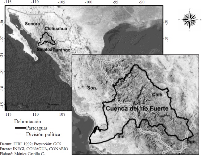
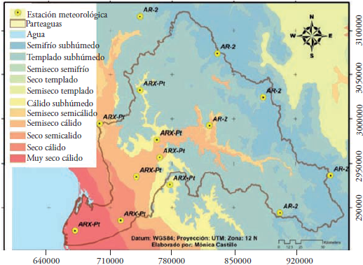
The Fuerte river watershed is located in the northwest of Mexico, in the states of Sinaloa, Sonora, Durango and Chihuahua (Figure 1), as part of the hydrological region Number 10, Sinaloa, between 25.68° and 28.24 ° N, and 106.12 ° to 109.43 ° W, with an area of 36 456 km2. Altitudes in the watershed range from 3168 to -9 masl (INEGI, 2014); its average annual precipitation is 691 mL and average temperature of 19.4 °C, according to the climatological normal values of 14 stations within the watershed, from 1961 to 2011 (SMN, 2014).
The watershed is born in the Sierra Madre Occidental and flows into the north of Sinaloa in the Gulf of California. The Rarámuri indigenous ethnic group inhabits the upper part of the watershed; it is a zone of high marginalization that in the last decade had serious drought problems; the Valle del Fuerte is located in the middle and lower part, which is an important agricultural area of production of grains and vegetables for the national and international market. The Fuerte river watershed is important due to its surface extension, the volume of its runoff and the dams Miguel Hidalgo and Costilla, Luis Donaldo Colosio and Josefa Ortiz de Dominguez, which are used to generate electricity and are the main source of water for agricultural, urban and industrial use.
Climatological information
The climatological information used for the calculation of the SPI and SPEI drought indices was obtained from the national meteorological service database available online (SMN, 2014). Besides, we used the monthly precipitation data (Pt), minimum temperature (Tmin) and maximum temperature (Tmax) of 14 weather stations during the period 1961-2011, which was the most complete and updated during this study.
The stations selected are distributed throughout the watershed; the most incomplete information was that of precipitation and on average 8 % of the rainfall missing data was generated (Table 1). In Batopilas, Chihuahua, one of the most extreme cases, 29 % of the rainfall data were generated. To generate the rain data, we used the inverse square distance method, and the details appear in an article for which the indices were generated (Castillo et al., 2017).
Table 1 Selected meteorological stations of the watershed.
| Clave | Estación | Altitud (msnm) |
Pt. media (mm) |
T. Mín. (°C) |
T. Máx. (°C) |
Periodo | % Datos generados |
| 8038 | Creel, Chihuahua | 2348 | 648.7 | 1.7 | 20.2 | 1961 - 2011 | 10.8 |
| 8106 | Norogachic, Chihuahua | 2088 | 578.8 | 2.7 | 21.6 | 1961 - 2011 | 20.7 |
| 8161 | Batopilas, Chihuahua | 678 | 603.4 | 16.7 | 31.3 | 1961 - 2011 | 29.4 |
| 8167 | Chinipas, Chihuahua | 440 | 838.2 | 16.0 | 31.0 | 1961 - 2011 | 2.6 |
| 8172 | Guadalupe, Chihuahua | 2279 | 1083.2 | 4.0 | 22.3 | 1961 - 2011 | 2.9 |
| 8182 | Moris, Chihuahua | 754 | 627.8 | 11.0 | 29.4 | 1961 - 2011 | 3.1 |
| 8267 | El Vergel, Chihuahua | 2740 | 629.7 | 0.6 | 17.6 | 1961 - 2012 | 24.8 |
| 25009 | Bocatoma, Sinaloa | 31 | 456.6 | 17.0 | 33.0 | 1961 - 2012 | 2.6 |
| 25019 | Choix II, Sinaloa | 239 | 707.0 | 14.2 | 34.2 | 1961 - 2012 | 1.9 |
| 25025 | P. Miguel H., Sinaloa | 144 | 619.8 | 16.6 | 33.8 | 1961 - 2012 | 1.3 |
| 25042 | Higuera, Sinaloa | 10 | 307.1 | 17.3 | 31.5 | 1961 - 2012 | 7.9 |
| 25044 | Huites, Sinaloa | 269 | 812.7 | 16.4 | 34.8 | 1961 - 2012 | 2.4 |
| 25100 | Yecorato, Sinaloa | 400 | 796.1 | 13.5 | 34.9 | 1961 - 2012 | 6.1 |
| 26053 | Minas N., Sonora | 480 | 672.4 | 15.0 | 31.2 | 1961 - 2011 | 5.7 |
Methodology
The meteorological, hydrological and agricultural droughts are represented by the drought index, which is a variable to assess the effect of a drought and includes intensity, duration, severity and spatial extension (Mishra and Singh, 2010). The SPI (McKee et al., 1993) is one of the most used for the detection and monitoring of droughts and is based on the probability of precipitation at any time scale to quantify the precipitation deficit (Velasco et al., 2004).
The SPEI (Vicente et al., 2010), in addition to the precipitation used by the SPI, considers the reference evapotranspiration (ET0) based on the monthly water balance (Pt-ET0), combining characteristics of the Palmer Drought Severity Index (PDSI) sensitivity and the simplicity of calculation, and the multi-temporal nature of SPI. It is very suitable to detect, monitor and explore the consequences of global warming in drought conditions (Vicente et al., 2010).
The SPI and SPEI indices were developed for the 14 selected stations, at scales of 3, 6, 12 and 24 months. The SPI series were generated with the spi_sl_6.exe program developed by the National Drought Mitigation Center (NDMC, 2014), and the SPEI was obtained with SPEI.R developed by Beguería and Vicente (2014) for the R/RStudio program.
In the SPEI calculation, the reference evapotranspiration method of Hargreaves-Samani was contemplated (Beguería et al., 2014). For more information on obtaining SPI and SPEI, and their interpretation as indicators of drought, consult Castillo et al. (2017), who detail the SPI and SPEI process in the watershed for our study.
In our study, the forecast of meteorological droughts was made by mixing autoregressive time series models with the Discrete Kalman filter (Kalman, 1960), which is a set of mathematical equations to estimate the state of a process minimizing the mean of the quadratic error. The Kalman filter operates by means of a prediction and correction mechanism, the algorithm predicts the new state from a previous estimate, adding a correction term proportional to the prediction error, minimizing it statistically (Welch and Bishop, 2006).
Autoregressive models are used in hydrology and meteorology because they are time dependent and easy to use (World Meteorological Organization, 2011). In our study, we proposed the creation of two autoregressive models, one of second order (AR2) and the other of second order with exogenous input (ARX) to forecast the future monthly states of the SPI and SPEI drought indices based on the previous records of the series. The choice of autoregressive models will be shown in Table 2 of Results and Discussion.
Table 2 Results in the SPI forecast for values of na and nb.
| Modelo | Índice | na | Nb | MSE | RMSE | E | R | PBE |
| DKF - AR (2) | SPI 12 meses | 2 | -- | 0.15 | 0.38 | 0.848 | 0.92 | -7.4 % |
| DKF - ARX (Pt) |
2 | 1 | 0.15 | 0.38 | 0.849 | 0.92 | -7.4 % | |
| 2 | 2 | 0.10 | 0.32 | 0.888 | 0.94 | 26 % | ||
| 2 | 3 | 0.10 | 0.32 | 0.887 | 0.94 | 35 % | ||
| 1 | 2 | 0.11 | 0.32 | 0.884 | 0.94 | 35 % | ||
| 3 | 1 | 0.10 | 0.32 | 0.889 | 0.94 | 23 % | ||
| 3 | 2 | 0.10 | 0.32 | 0.889 | 0.94 | 30 % | ||
| 3 | 3 | 0.10 | 0.32 | 0.888 | 0.94 | 40 % | ||
| 4 | 1 | 0.10 | 0.32 | 0.889 | 0.94 | 20 % | ||
| 4 | 2 | 0.10 | 0.32 | 0.889 | 0.94 | 26 % | ||
| 4 | 3 | 0.10 | 0.32 | 0.887 | 0.94 | 30 % | ||
| 4 | 4 | 0.10 | 0.32 | 0.887 | 0.94 | 31 % |
The AR2 and ARX models (equations 1 and 2, respectively) relate the input of the system to its output by means of a linear equation in differences with constant coefficients:
where y t is the observed value of the index at time t, which represents one month; rt is the value of the exogenous variable (Pt, Tmin, Tmax, ET0) at time t; et+1 is the error term in the index estimate; αi and βi are parameters; the indices na and nb specify the number of previous observations of the index and exogenous variables, respectively. From the general structure of both autoregressive models, the formulation in a state space allows to use them within the algorithm of the Discrete Kalman filter as follows:
where x k+1 is the value of the index (not observed) of size (n x 1); A is the matrix of αi size parameters (n x n); x k is the index in time k of size (n x 1); B is the matrix of βj exogenous size parameters (n x m); vk is the vector that contains the exogenous variable registered for time k; zk is the index in time k of size (m x 1); H is the transformation matrix that maps the state vector to the domain of the measurement with dimensions (m x n);W k and vk are vectors representing Gaussian noise in the process and noise in the measurement for each observation with sizes (m x 1), and it is expected that such Gaussian noises are distributed in a normal way with mean 0 and Q and R variances, respectively :
According to Simon (2001), there is no correlation between Q and R, that is, they are independent random variables and can vary over time, but they are assumed constant for simplicity, and it is defined as:
where Q is the covariance matrix of the system disturbance;
R is the covariance matrix of the measurement
perturbation;
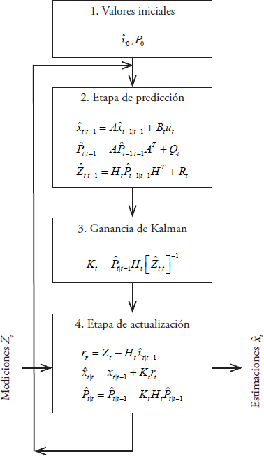
The matrix R is (1 x 1) and contains the expected error of the measurements, defined as a proportion (α) of the previous measurement, so R=α*(xk -1), in this specific case α=0.001; higher values generate extreme data that are located outside the range in which values of drought indices normally present, reducing the prediction power of the model. With respect to the size of the matrices, the value of n is equal to na, and the value of m equal to nb; where na and nb indicate the number of previous observations of the index and the exogenous variables, respectively. The algorithm of the Discrete Kalman filter is described in Figure 2.
To create the AR and ARX models, we programmed routines in Matlab® (Math Works 2015), to obtain the values of the parameter matrices in line with the order of the autoregressive process according to equations 1 and 2. The ARX was also an autoregressive model of second order, but with exogenous variable.
Since the behavior of the drought in the watershed varies depending on the occurrence of the rainy season and phenomena such as El Niño or La Niña, among other global climatic phenomena, the parameters estimated for the AR and ARX models were recalculated after a certain time period (P) to obtain more representative forecasts of the previous conditions of humidity in each station. The forecast began in the period (t0 + P) until the time (t0 + 2P), in this point we recalculated the parameters of the models according to period [P: 2P], and so on until ending with the last data group. Thus, the implementation of DKF - AR2 and DKF - ARX became dynamic and incorporated the climatic changes that occurred in the watershed during the study period of each season or certain period.
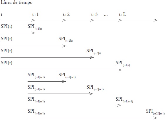
We did the forecast of the SPI and SPEI indices at four-time scales for each station, and implemented the AR2 and ARX models (Pt, Tmin, Tmax and ET0 as exogenous variables) with the Discrete Kalman filter. To know the effectiveness of the models in the forecast for L steps forward, that is, with 1, 2, 3 and 4 months in advance, we created a routine in Matlab® to perform the forecast considering the information in time k and advance L steps in the forecast without updating the information (Figure 3); we conducted this process considering the P period of calibration of the AR2 and ARX models.
To evaluate the results of the forecast, we calculated the main statistics according to Gupta et al. (2009); the RMSE (the root of the mean square error) and E (the Nash-Sutcliffe efficiency) were the criteria to be considered as they are the most used for the calibration and evaluation of hydrological models (Moriasi et al., 2007). In addition, a 95% confidence interval was included that follows the route of each state of the series with the objective of establishing the degree of uncertainty associated with the forecast at each time step (L) with respect to the values observed.
The prediction interval (I.P.) was obtained according to the criteria established by Chatfield (2004), the I.P. was calculated based on the following general form: 100(1-α)% I.P. for xt+L is given by:
where
Results and discussion
In its process the Kalman filter generates two types of results: the predicted and updated states, the results will only include the forecast part since based on this the performance of the models will be evaluated to predict the future states of the drought indices.
The results are presented in the forecast of the SPI and SPEI drought indices in the Fuerte river watershed, implementing the DKF - AR2 and DKF - ARX models with information from 14 meteorological stations in the period from 1961 to 2011.
The na and nb indices were assigned the values of na = 2 and nb = 2, to generate the best results in terms of RMSE and E with the lowest possible number of observations (Table 2). Figure 4 shows that the calibration period for both models was 96 months. The calibration period was established to estimate and re-estimate the parameters of the model during the study, since the characteristics of the drought can vary over time and have a cyclical or seasonal behavior. Different periods between 60 and 108 months (less than 10 years) were tested, a range within which we can see some recurrent behavior of the drought indices and, besides, there is enough information to estimate the parameters of the model without considerably reducing the series available to make the forecast. Table 3 shows the results for each calibration period in terms of RMSE and E, where we deduced that the most appropriate period is 96 months.
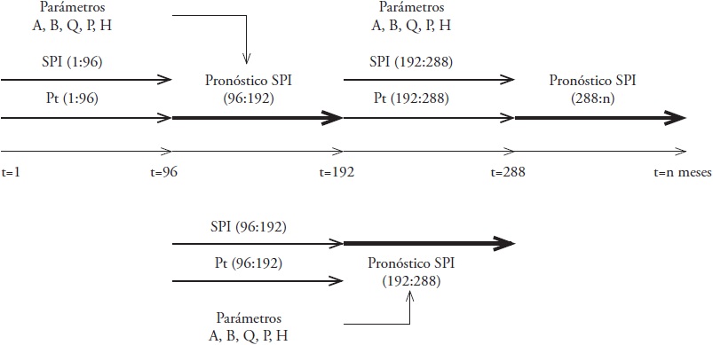
Table 3 Test of different calibration periods for station 25025 P. Miguel Hidalgo, Sinaloa.
| Modelo | Periodo de calibración (meses) | |||||||||
| DKF - ARX-Pt | 60 | 72 | 84 | 96 | 108 | |||||
| RMSE | 0.37 | 0.37 | 0.37 | 0.36 | 0.37 | |||||
| E | 0.855 | 0.860 | 0.857 | 0.868 | 0.869 | |||||
The statistics selected to describe the results of this study is the RMSE which is expressed in the units of the indices and was taken into account because the error made in the forecast defines the effectiveness of the model to make predictions and thus whether it is a suitable tool, otherwise other forecasting methods may be chosen. The second parameter is E, the Nash efficiency coefficient, which according to Moriasi et al. (2007), depending on the values of E, it would be the quality of the prediction of the model (E<0.5 the model is unsatisfactory and when approaching 1 it is a good model). These values arise from a relation between the data observed of the index and those that the forecast throws with the algorithm of the Discrete Kalman filter; in this relation the value of E indicates the degree in which the DKF - AR2 and DKF - ARX models are better predictors than the mean of the observed data (given that E>0.5). Therefore, it is considered one of the parameters for evaluating the forecast given by drought indices.
Tables 4 and 5 show the mean values of the RMSE and E statistics obtained in the forecast of the SPI and SPEI indices for the 14 stations analyzed. These results are presented by the time scale of the indices and by the models used, models DKF - AR2 and DKF - ARX- (Pt, ET0, Tmin, Tmax).
Table 4 Mean of the results in the SPI forecast in the watershed.
| Duración de la sequía en meses | ||||||||
| Modelo | 3 | 6 | 12 | 24 | ||||
| RMSE | E | RMSE | E | RMSE | E | RMSE | E | |
| AR-2 | 0.67 | 0.50 | 0.53 | 0.70 | 0.34 | 0.88 | 0.24 | 0.94 |
| ARX-Pt | 0.68 | 0.51 | 0.46 | 0.78 | 0.32 | 0.89 | 0.21 | 0.95 |
| ARX-ET0 | 0.70 | 0.48 | 0.46 | 0.78 | 0.32 | 0.89 | 0.21 | 0.95 |
| ARX-TMIN | 0.70 | 0.49 | 0.46 | 0.78 | 0.32 | 0.89 | 0.21 | 0.95 |
| ARX-TMAX | 0.70 | 0.48 | 0.47 | 0.78 | 0.32 | 0.89 | 0.21 | 0.95 |
Table 5 Mean of the results in the SPEI forecast in the watershed.
| Duración de la sequía en meses | ||||||||
| Modelo | 3 | 6 | 12 | 24 | ||||
| RMSE | E | RMSE | E | RMSE | E | RMSE | E | |
| AR-2 | 0.65 | 0.58 | 0.48 | 0.76 | 0.30 | 0.90 | 0.21 | 0.96 |
| ARX-Pt | 0.63 | 0.61 | 0.43 | 0.81 | 0.27 | 0.92 | 0.19 | 0.96 |
| ARX-ET0 | 0.64 | 0.59 | 0.44 | 0.81 | 0.27 | 0.92 | 0.19 | 0.96 |
| ARX-TMIN | 0.64 | 0.60 | 0.44 | 0.81 | 0.27 | 0.92 | 0.19 | 0.96 |
| ARX-TMAX | 0.65 | 0.58 | 0.44 | 0.81 | 0.27 | 0.92 | 0.19 | 0.96 |
The 3- and 6-month time scales in both indices obtained RMSE means between 0.40 and 0.70; the SPI and SPEI change category every 0.50 units, so errors of this magnitude mean a wide margin of error in the prediction of the indices that can lead us to underestimate the intensity of drought or humidity conditions. In contrast, the time scales of 12 and 24 months obtained average values of RMSE between 0.19 and 0.34, which generates a better approximation to the real conditions in the watershed.
The coefficient E, in the 3-month SPI forecast, presents mean values less than and equal to 0.5, classifying the models as unsatisfactory for these conditions; while the SPEI for the same time scale presents mean values of E assessed as satisfactory. The SPI and SPEI forecast at time scales of 6, 12 and 24 months obtained mean values of E greater than 0.70, classifying the five models tested as good and very good, therefore, despite the magnitude of the errors committed at the 6-month scale, the models are better predictors than the mean of the data observed.
In general terms of RMSE and E, the SPEI forecast is better than the SPI forecast for the tested models and at all time scales. This may be due to the fact that the SPEI involves two variables in its calculation: precipitation, which is a variable of a more random character (spatially and temporally) than temperature, so that the temperature variable gives greater stability to the SPEI series, improving the prognosis; on the other hand, the SPI uses only precipitation for its calculation, which generates high variability in the data series and increases the error made in the forecast of the index, as shown in Tables 4 and 5.
From Tables 4 and 5, we concluded that the SPEI forecast for the 12 and 24-month scales generates better results than the 3 and 6-month scales, in terms of the RMSE and E for the autoregressive models tested.
Table 6 shows the model that generated the best results in the forecast with the Discrete Kalman filter of the SPEI of 12 and 24 months. We observed that in 6 of the 7 stations that are located in the state of Chihuahua, in the upper part of the watershed, the best model is the second-order autoregressive AR2, which uses only the monthly data series of the SPEI. The remaining 8 stations, most of them located in the north of Sinaloa, presented better results with the autoregressive model with exogenous input of precipitation ARX-Pt. Among the exogenous variables analyzed (precipitation, reference evapotranspiration and maximum and minimum temperatures), precipitation was the one with the lowest RMSE and the highest value of E in all stations.
Table 6 Best forecast models of the SPEI with the DKF for each station.
| Clave | Estación | Mejor modelo de pronóstico | Duración de la sequía | |||
| 12 | 24 | |||||
| RMSE | E | RMSE | E | |||
| 8038 | Creel | AR-2 | 0.27 | 0.92 | 0.19 | 0.97 |
| 8106 | Norogachic | AR-2 | 0.27 | 0.92 | 0.19 | 0.97 |
| 8161 | Batopilas | AR-2 | 0.28 | 0.91 | 0.16 | 0.97 |
| 8167 | Chinipas | ARX-Pt | 0.27 | 0.92 | 0.19 | 0.96 |
| 8172 | Guadalupe | AR-2 | 0.26 | 0.94 | 0.16 | 0.98 |
| 8182 | Moris | AR-2 | 0.17 | 0.97 | 0.10 | 0.99 |
| 8267 | El Vergel | AR-2 | 0.27 | 0.91 | 0.17 | 0.96 |
| 25009 | Bocatoma | ARX-Pt | 0.27 | 0.92 | 0.19 | 0.96 |
| 25019 | Choix | ARX-Pt | 0.27 | 0.92 | 0.19 | 0.96 |
| 25025 | P. Miguel H. | ARX-Pt | 0.27 | 0.92 | 0.19 | 0.96 |
| 25042 | Higuera | ARX-Pt | 0.27 | 0.92 | 0.19 | 0.96 |
| 25044 | Huites | ARX-Pt | 0.27 | 0.92 | 0.19 | 0.96 |
| 25100 | Yecorato | ARX-Pt | 0.27 | 0.92 | 0.19 | 0.96 |
| 26053 | Minas Nuevas | ARX-Pt | 0.27 | 0.92 | 0.19 | 0.96 |
In the SPEI forecast at 12- and 24-month durations, we observed that a single model cannot generate the best results for all the stations in the watershed, but both models can be good forecasting tools based on specific characteristics of the data series of the stations.
Figure 5 shows the model that was the best predictor in each meteorological station and its probable association with the climatic units that predominate in each zone. It is worth noting that the stations in which the inclusion of an exogenous variable did not improve the forecast are located in semi-cold and temperate climates; whereas the stations in which the ARX-Pt model was the best forecast model are located in dry and warm climates. In these stations the inclusion of precipitation as an exogenous variable improved the SPEI forecast and gave more information to the algorithm.
This difference in the best forecast model for temperate and warm weather stations is due to the characteristics of the SPEI series of each station. Figure 6 shows two series of the 12-month SPEI, the first series of station 8172 Guadalupe located in a temperate climate, and the second of station 25100 Yecorato, which is in a warm climate. The figure shows some parts of the series where it is clear that the number of oscillations of SPEI in Guadalupe is much lower than in Yecorato. Remember that from drought indices of -1.0 the classification of moderate drought begins (Castillo et al., 2017), and that the more negative the index, the greater the drought.
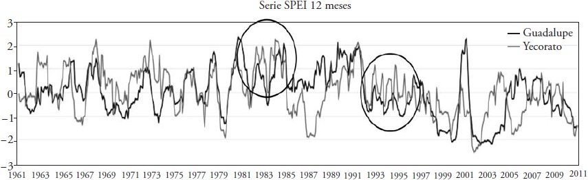
Table 6 Comparison between the SPEI series of 12 months of a temperate climate station (Guadalupe, Chihuahua) and a warm climate station (Yecorato, Sinaloa).
Similarly, Figure 7 shows two series of the 12-month observed SPEI (line) and the predicted value (asterisk). The upper series corresponds to station 8106 Norogachic, of temperate climate; its predicted value was obtained with the model AR2, and it is possible to appreciate how the prediction fits the series observed, especially in the extreme values.
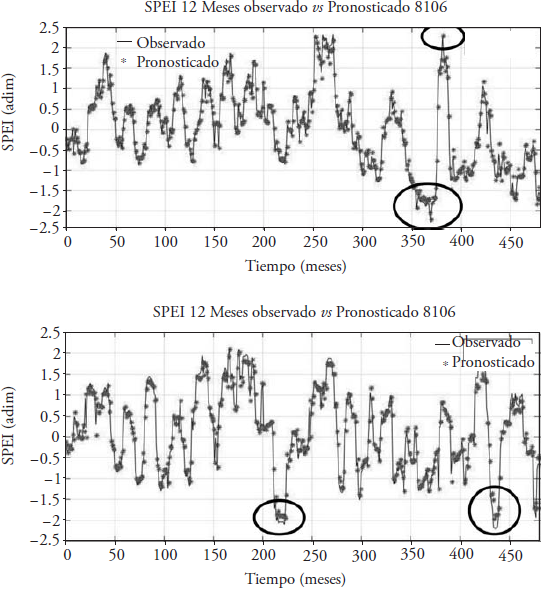
Figure 7 SPEI series of 12 months observed and predicted from a station located in cold weather (8106, Norogachic) and another in a warm climate (25025, P. Miguel Hidalgo).
The lower series corresponds to the station 25025 Presa Miguel Hidalgo, located in warm weather; the best forecast was obtained with the ARX-Pt model, and unlike the temperate climate station, the prediction does not have an adequate adjustment to the extreme values.
Forecast with DKF - ARX-Pt
In stations 8167, 25009, 25019, 25025, 25042, 25044, 25100 and 26053 (6 of them are in Sinaloa), we obtained better results in the SPEI forecast with the DKF-ARX-Pt model. The results showed that the use of precipitation as an exogenous variable improves the forecast compared to the one made with the DKF-AR2 model for these stations.
With the ARX model, precipitation, reference evapotranspiration, maximum and minimum temperature were tested as exogenous variables; however, in most cases precipitation contributed more information to the algorithm and generated better results in terms of E and R than the remaining variables (Table 6).
The association of the results with the climatic units of the watershed locates these stations in hot and dry climates. As already shown, the hot weather stations show series with greater oscillation between positive and negative values of the SPEI than the series of stations in temperate and semi-cold climates. By having less smoothed series the forecast becomes less precise, so the inclusion of an exogenous variable (precipitation) provides the necessary information to the model to improve its performance.
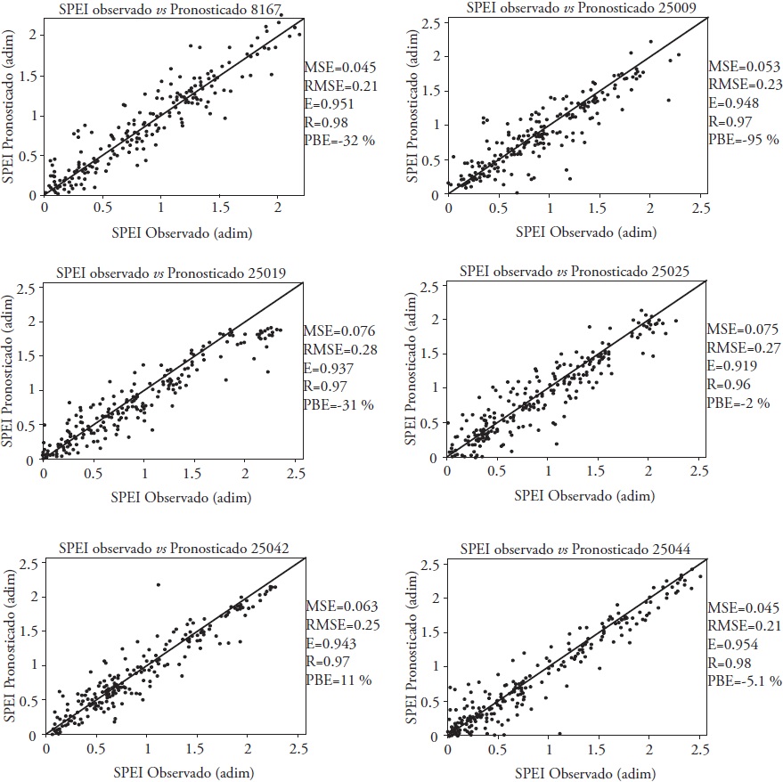
Figures 8 and 9 show the dispersion diagrams of SPEI of 12 and 24 months, respectively, for the stations where the ARX-Pt model was better. These Figures show the values of MSE, RMSE, E, R and PBE.
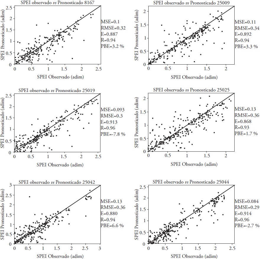
Figure 8 Dispersion diagrams of observed and predicted values of 12-month SPEI for some stations where ARX-Pt was the best model.
Forecast with DKF - AR2
The stations 8038, 8106, 8161, 8172, 8182 and 8267, all located in the state of Chihuahua on the Sierra Madre Oriental, obtained better results in the SPEI forecast with the DKF-AR2 model (Table 6). In these stations the inclusion of an exogenous variable such as precipitation, reference evapotranspiration, maximum and minimum temperature did not provide enough information to the algorithm to improve the results obtained with the AR2 model; if anything, it matched them.
The association of the results with the type of climate of the station locates these stations in semi-cold and temperate semi-humid climates.
The value of the PBE (Percentage Bias Error) statistic is negative in most stations, which indicates that the model DKF-AR2 underestimates the value of the SPEI index (Table 6).
In both forecast models of the SPEI, DKF-AR and DKF-ARX, the 12-month series show higher error and lower value of the Nash coefficient than the 24-month series; this is due to the fact that on a larger scale the time series assimilates more slowly the changes given in the balance Pt-ET0 over time, and therefore presents more smoothness in its route, improving the forecast.
However, both forecasts of droughts of 12 and 24-month duration are useful. But given the characteristics of the drought indices (SPI and SPEI) at a certain scale (duration of drought), in terms of operability, the 12-month time scale is considered the most appropriate for the forecast of droughts. The latter is particularly suitable in the middle and lower parts of the watershed due to its agricultural and energy values, where annual policies of operation are analyzed when operating the dams, although the analysis of drought periods of 24 months is very useful as well.
In addition to the forecast of the drought index for the time t+1|t, we predicted the indices with 2, 3 and 4 months in advance; that is, given an observed value of the index in time t, we predicted the index values for the time t+1, t+2, t+3 and t+4 without updating the information, with the purpose of knowing the power of prediction of the models for different steps of advancement in time. However, as a sample, we present here only the forecast results for the 12-month SPEI. Figure 10 shows the forecast at the Miguel Hidalgo Dam station in Sinaloa, with the 12-month SPEI using the DKF-ARX-Pt model with 1, 2, 3 and 4 months in advance.
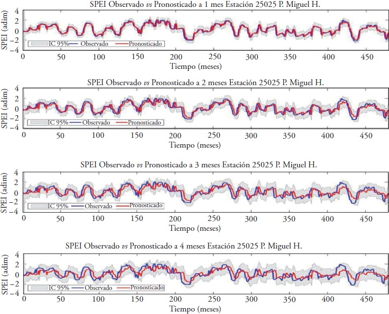
Figure 10 The 12-month SPEI predicted with the DKF-ARX-Pt model with 1, 2, 3 and 4 months of anticipation and 95% confidence interval, Presa Miguel H. station, Sinaloa.
The forecast focuses on the point estimate of a 12-month SPEI value for some future month, but according to Chatfield (2004): “the point forecast is adequate for many purposes, but a prediction interval is often very helpful to give a better indicator of future uncertainty”. Therefore, we calculated the confidence interval of the forecast at 95 % for the advance steps (L), as indicated in equation (9).
In Figure 10, in addition to the observed and predicted values, there is a stripe that follows the forecast path (the more negative the index, the greater the drought), and this is the confidence interval of the forecast at 95 %. As the forecast progresses, the interval becomes wider. For example, at time t there is less uncertainty from where the observed value of the SPEI can be located at time t+1 than from the value at time t+4 in which uncertainty is much greater.
It is also important to add that in the end we observed how the total errors of the prediction (of the process + of measurement) were adjusted to a t-Student distribution of mean 0, which approaches a normal distribution.
It is worth emphasizing that the Kalman filter is important for the forecast of hydrometeorological variables because daily mean flows can be predicted (Gonzalez et al, 2015), as well as sub-hourly flows (Morales et al., 2014), and predict indicators of droughts with some months of anticipation. The prediction of droughts allows preparing contingency plans to reduce their negative impact.
Conclusions
The forecast of SPI and SPEI drought indices using the discrete Kalman filter and two autoregressive models, AR2 and ARX, was successfully implemented for 14 meteorological stations in the Fuerte river watershed in the period 1961-2011. The AR2 model presented better adjustments for the upper part of the watershed and the ARX, for the middle and lower part of it. As external variables in the ARX model, we tested the following variables: precipitation, reference evapotranspiration, maximum temperature and minimum temperature.
The external variable in the ARX model that improved the prediction was precipitation. Other studies recommend to include the previous moisture condition in the watershed as an external variable.
It is important not only to monitor droughts with improved indices such as the SPEI, but also to predict them ahead of time in order to carry out contingency plans for the demands of drinking, agricultural and livestock water. The Discrete Kalman filter was a good tool for forecasting droughts. This is the main contribution of this research.
Literatura citada
Al-Qinna, M. I., N. A. Hammouri, M. M. Obeidat, and F. Y. Ahmad. 2011. Drought analysis in Jordan under current and future climates. Climatic Change 106: 421-440. [ Links ]
Beguería, S., and F. Vicente. 2014. Calculation of the Standardized Precipitation-Evapotranspiration Index. Package SPEI. R for R or RStudio Program. https://cran.r-project.org/web/packages/SPEI/SPEI.pdf (Consulta: marzo 2014). [ Links ]
Beguería, S., S. M. Vicente‐Serrano, F. Reig, and B. Latorre. 2014. Standardized precipitation evapotranspiration index (SPEI) revisited: parameter fitting, evapotranspiration models, tools, datasets and drought monitoring. International J. Climatol. 34: 3001-3023. [ Links ]
Castillo-Castillo, M., L. A. Ibáñez-Castillo, J. B. Valdes, R. Arteaga-Ramírez, y M. A. Vázquez-Peña. 2017. Análisis de sequías meteorológicas en la cuenca del río Fuerte, México. Rev. Tecnol. Ciencias del Agua 8: 35-52. [ Links ]
Chatfield, C. 2004. The Analysis of Time Series: An Introduction. Six edition. Chapman &Hall/ CRC Press. 313 p. [ Links ]
Dehghani, M., B. Saghafian, F. Nasiri Saleh, A. Farokhnia, and R. Noori. 2014. Uncertainty analysis of streamflow drought forecast using artificial neural networks and Monte‐Carlo simulation. Int. J. Climatol. 34: 1169-1180. [ Links ]
Eicker, A., M. Schumacher, J. Kusche, P. Döll, and H. M. Schmied. 2014. Calibration/data assimilation approach for integrating GRACE data into the WaterGAP Global Hydrology Model (WGHM) using an ensemble Kalman filter: First results. Surveys in Geophysics 35: 1285-1309. [ Links ]
González-Leiva, F., L. A. Ibáñez-Castillo, J. B. Valdés, M. A. Vázquez-Peña, y A. Ruiz-García. 2015. Pronóstico de caudales con el filtro de Kalman en el río Turbio. Tecnol. Ciencias del Agua 6: 5-24. [ Links ]
Gupta H. V., H. Kling, K. Yilmaz, G.F. Martinez. 2009. Decomposition of the mean squared error and NSE performance criteria: Implications for improving hydrological modelling. J. Hydrol. 377: 80-91. [ Links ]
Instituto Nacional de Estadística y Geografía, INEGI. 2014. Continuo de Elevaciones Mexicano 3.0, CEM 3.0. inegi.org.mx/geo/contenidos/datosrelieve/continental/continuo-elevaciones.aspx ]. (Consulta: enero 2014). [ Links ]
Kalman, R. E. 1960. A new approach to linear filtering and prediction problems. J. Fluids Eng. 82: 35-45. [ Links ]
Kim, T., J. B. Valdés, and J. Aparicio. 2002. Frequency and spatial characteristics of droughts in the Conchos River Basin, Mexico. Water Int. 27:420-430. [ Links ]
Kim, P. 2011. Kalman Filter for Beginners: with Matlab Examples. Seoul, Korea: CreateSpace. 232 p. [ Links ]
Madadgar, S., and H. Moradkhani. 2013. A Bayesian framework for probabilistic seasonal drought forecasting. J. Hydrometeorol. 14: 1685-1705. [ Links ]
MathWorks, Inc. 2015. Software Matlab® [ Links ]
McKee, T. B., N. J. Doesken, and J. Kleist. 1993. The relationship of drought frequency and duration to time scales. Eight Conference on Applied Climatology. Anaheim, CA, American Meteorological Society. 179-184. [ Links ]
Mishra, A. K., and V. P. Singh. 2010. A review of drought concepts. J. Hydrol. 391: 202-216. [ Links ]
Mishra, A. K., and V. P. Singh. 2011. Drought modeling-A review. J. Hydrol. 403: 157-175. [ Links ]
Morales-Velázquez, M. I., J. Aparicio, and J. B. Valdés. 2014. Pronóstico de avenidas utilizando el Filtro de Kalman Discreto. Tecnol. Ciencias del Agua 5: 85-110. [ Links ]
Moriasi, D., N., J. G. Arnold, M. W. Van Liew, R. L. Bingner, R. D. Harmel, and T. L. Veith. 2007. Model evaluation guidelines for systematic quantification of accuracy in watershed simulations. Soil & Water Division of ASABE 50: 885-900. [ Links ]
Mossad, A., and A. A. Alazba. 2015. Drought forecasting using stochastic models in a hyper-arid climate. Atmosphere 6: 410-430. [ Links ]
National Drought Mitigation Center, NDMC. 2014. SPI SL 6.exe: Program to calculate Standardized Precipitation Index. http://drought.unl.edu/MonitoringTools/-DownloadableS-PIProgram.aspx ]. (Consulta: febrero 2014). [ Links ]
Ravelo, A. C., R. Sanz-Ramos, and J. C. Douriet-Cárdenas. 2014. Detección, evaluación y pronóstico de las sequías en la región del Organismo de Cuenca Pacífico Norte, México. Agriscientia 31: 11-24. [ Links ]
Rhee, J., and J. Im. 2017. Meteorological drought forecasting for ungauged areas based on machine learning: Using long-range climate forecast and remote sensing data. Agric. Forest Meteorol. 237: 105-122. [ Links ]
Servicio Meteorológico Nacional. 2014. Climatología Diaria. http://smn.cna.gob.mx/-es/climatologia/informacion-climatologica . (Consulta: enero 2014). [ Links ]
Simon, D. 2001. Kalman filtering. Embedded Systems Programming 14: 72-79. [ Links ]
Velasco, I., J. Aparicio, J. B. Valdés, J. Velázquez, y T. Kim. 2004. Evaluación de índices de sequía en las cuencas de afluentes del río Bravo/Grande. Ing. Hidrául. México 19: 37-53. [ Links ]
Vicente, S. S, S. Beguería, and M. J. López. 2010. A multiscalar drought index sensitive to global warming: the standardized Precipitation Evapotranspiration Index. J. Climate. 23: 1696-1718. [ Links ]
Welch, G., and G. Bishop. 2006. An Introduction to the Kalman Filter. Department of Computer Science, University of North Carolina, Chapel Hill. 16 p. https://www.cs.unc.edu/~welch/media/pdf/kalman_intro.pdf (Consulta: octubre 2018). [ Links ]
World Meteorological Organization, WMO. 2011. Guide to Hydrological Practices. Sixth Edition. Geneva, Swiss. 330 p. [ Links ]
Received: March 2017; Accepted: November 2017
 Este es un artículo publicado en acceso abierto bajo una licencia Creative Commons
