Study area

The evaluated plantations was of E. urophylla, with cultural activities, without silvicultural intervention and an initial density of 1100 plants per ha. It is located in the municipality of Huimanguillo, Tabasco, Mexico (17° 55’ N, 94° 06’ W, 30 m mean altitude). The region has rain and dry seasons, with warm, humid climate (Am), mean annual temperature of 26 °C and 2,500 mm precipitation. The soils are Feozem type with a hill relief type (^{INEGI, 2005}).

Sample selection and assessment

A random sampling was carried out in seven dispersed E. urophylla plantations, in which 93 clonal trees, one to seven years old, were destructively sampled. These were selected by their top morphological condition in the plantations. This sampling tried to cover the span of trees growth and age variability. On each tree, before timbered, we measured diameter at breast height (dn), and after being fell, their total height (AT), stump diameter and height (dt and Atc), basal diameters (db) per branch and at the bole insertion height (Adb). All measurements were recorded in meters.

Component separation

Bole with bark, branches, and foliage were separated and weighed to obtain the green weight (Fw, in kg), following the methodology proposed by ^{Avendaño-Hernández et al. (2009)} and ^{Gómez-Díaz et al. (2011)}. We then sectioned the trunk in one-meter length logs, starting at stump-height up to the tip. Each section was weighed on an electronic platform scale (100 kg capacity with 0.001 kg precision). Three 5 cm thick slices were obtained stump, middle and tip of each tree trunk. Branches and foliage were then separated and weighed on an electronic scale (5 kg capacity, 0.001 kg precision). A sample of branches and foliage, about 0.5 kg, was selected to determine the relationship between green and dry weight. The latter determined in a laboratory. We followed the methodology documented by ^{Ruíz-Aquino et al. (2014)} and ^{Soriano-Luna et al. (2015)}.

Bark and aerial biomass volume estimation

We calculate the volume of each log or section (Vlog) with the Newton formula and the tip volume (Vtip) with the cone volume formula. The total tree volume (Vt) was calculated using the overlapping log method proposed by ^{Bailey (1995)}. The samples of the branches and leaves were dehydrated in a drying oven at 72 °C and the slices at 105 °C until constant weight was reached. The weights were then recorded with an accuracy of 0.001 kg. Wet and dry weight determined the moisture content per component and the relationship between them. The total aereal biomass was the sum of the dry weight of the three components (^{Domínguez-Cabrera et al., 2009}; ^{Lim et al., 2013}). In addition, the average biomass proportion per component was determined respect to the total biomass.

Exploratory analysis of the samples

An exploratory analysis of the dependent (B _s , B _b , B _f , B _t and V) and independent (dn and AT) variables showed the wide dimensional variability of the of individuals (Table 1).

Table 1 Basic statistical values of the variables of trees sampled in commercial forest plantations of Eucalyptus urophylla, with one to seven years of age in Huimanguillo, Tabasco, Mexico. 

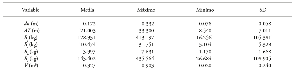
dn: diameter at breast height, AT: total height, Bs: bole biomass, Bb: branches biomass, Bf: foliage biomass, Bt: total biomass, V: volume, SD: mean standard deviation.

Fitting of biomass models and statistical analysis

Before the fitting, the data were normalized with the Shapiro-Wilk (SW) test (α=5 %). Here we propose that, if H ₀ is equal to or less than α, the information normality assumption is accepted, and the H ₁ rejected. If H ₁ was greater than the significance level of α, we would then conclude that the data was not normal, and the H ₁ accepted. In addition, to correct heteroskedasticity, a weighting function based on the combined variable (dn ² AT), as a weight in the residuals (α²=x _i ^k ) (^{Neter et al., 1996}; ^{Álvarez-González et al., 2007}): where α _i ² is the residual variance of the independent variable (x) and k is the optimization exponent value. The above consists in using the squared errors adjusted model without the ê _i ² weight as a dependent variable in the error variance potential model (^{Harvey, 1976}).

We tested linear and nonlinear models for the total biomass and by structural component (^{Loetsch et al., 1973}, ^{Segura and Andrade, 2008}, ^{Méndez-González et al., 2011}, ^{Gómez-García et al., 2013}). These models included dn and AT as independent variables. Also, we tested a general model that considers sd, sh, height and diameter of the clean shaft (Afl and dfl) and the summation of the basal diameters of all living branches in the tree (Σdb) (Table 2)

Table 2 Fitted models to estimate total biomass and by structural component 

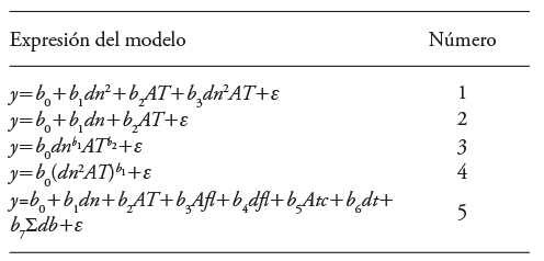
y: total biomass or by structural component, bi: parameters to be estimated, e: term of the model error.

Statistical fittings performed to equations 1 to 4 were by using the MODEL procedure in the SAS 9.2 statistical package using ordinary least squares (^{SAS Institute Inc., 2008}). Then based on the smallest values of the square root of the mean error (SMER) and the highest value of the coefficient of determination adjusted for the number of parameters (R ² a) the most efficient model was determined.

The four models, selected by structural component, simultaneously fitted as a system of seemingly unrelated equations. ^{Álvarez-Gonzáles et al. (2007)} considered it by including the y as endogenous or dependent variables and exogenous variables measured directly in the forest. In this way, the joined errors were included in the fitting, and consistent estimators obtained for the biomass components (^{Hernández et al., 2013}) in addition to the SMER, R ² a, significance parameters and approximate standard errors (EEa) fitting statistics (^{Alvarez-González et al., 2005}).

Model 5 included the sd, sh, Alf y dfl variables in addition to Σdb, and adjusted with the backward and forward selection methods, as recommended by ^{Volke (2008)}. Thus, the model only included the variables that explain the response variable with precision. The best-fit model selected with the already described goodness of fit criteria had the lower value in the Mallows Cp statistic, the highest R ² value, and F test partial significance.

The accuracy of the estimates of the total and structural biomass components of the best equations was evaluated through the bias and the aggregate difference in percentage, following ^{Barrero et al. (2015)}, and the formulas proposed by ^{Fonseca et al. (2009)}, ^{Lencinas and Mohr-Bell (2007)} and ^{Vargas-Larreta et al. (2010)}.

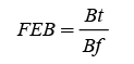
Biomass expansion factor (BEF)

We estimated the BEF in three ways. The first was through the total aerial biomass ratio and bole biomass (^{Dauber et al., 2002}). This allow to identify the distribution and changes in the tree aerial biomass structural components, or the species with the dimensions or as tree age increase. BEF was then estimated using equations 6 and 7 (^{Domínguez-Cabrera et al., 2009}; ^{Rodríguez-Ortiz et al., 2012}). The results were then added and averaged to define the BEF in the plantations by age (E) and diameter class (CD).

(6)

(7)

where B _S , B _f and B _b are: bole biomass, foliage biomass and branch biomass.

The second methodology to determine BEF considered the direct proportion of the volume (V, m³) respect to each tree shaft biomass and total biomass (kg). BEF allows identifying the volumetric stocks in the plantations in relation to the biomass. The factor was estimated with the structure studied by ^{Ruíz-Aquino et al. (2014)} for stem biomass (expression 8) and that proportion was calculated with total biomass using equation 9.

(8)

(9)

In the third method, in order to estimate the BEF, we defined the linear relationship of the biomass components with the volume, where the value multiplying the mean biomass volume (kg) per m³ that can be obtained. This relation represented in expressions 10 and 11, for total biomass and stem biomass, each.

(10)

(11)

where α ₀ and α ₁ are the parameters to be estimated and represent the total and bole biomass BEF, respectively.

BEF estimation methods comparison

The estimated by tree and population B _t and B _S averages were analyzed on a one-way ANOVA (^{Martínez-González et al., 2006}) to determine the existence of significant statistical differences. The hypotheses were: H ₀ =u ₁ =u ₂ =u ₃ . The means of the estimates are the same, accepting the equality hypothesis.H ₁ =at least one of the means is different, and therefore the equality hypothesis is rejected.

When the mean equality (u _k ) hypothesis by tree and population is contrasted, the decision rule that applied was based on the F significance in the Duncan (Pd) test, grouping the sample by method with 5 % significance.

Aerial biomass inventory

In order to observe the applicability of the results in a forest inventory and the BEF, three equations of total volume generated in the Huimanguillo, Tabasco, region in 2015 (12), 2012 (13) and 2007 (14) were compared and used in the clonal CFPs of E. urophylla for volume estimation.

(12)

(13)

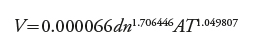(14)

To corroborate the applicability of the generated equations in a forest inventory, we performed an analysis with inventory data on a simple random sampling design. The inventory estimators were obtained from 28,500 m² rectangular sites, surveyed in 2014, in E. urophylla seven plantations. Plants were one to seven years old. The performed comparison of the results was an analysis of variance between the estimates with the t-Cramer test with 95 % confidence, to verify if the calculations were equal to each other.

Aerial biomass distribution

Biomass by structural component of the plantations had a mean of 43.0 %, 44.8 % and 37.8 % of harvest weight from the bole, branches, and foliage. The biomass distribution per component indicates that the proportion in the bole and its volume increased with the dn and TH increase. The opposite occurred with the proportion of branches and foliage biomass (^{Ferrere et al., 2008}, ^{Soriano-Luna et al., 2015}).

Eucalyptus urophylla clones trees established in CFP concentrated 92.42 % of the total biomass in the shaft, 5.54 % in the branches and 2.03 % in the foliage (Table 3). These results contrasted with those of ^{Cerruto et al. (2015)} on E. grandis plantations in Brazil, because at the age of 5.5 years, the proportion was 82 % for the bole and 18 % for branches, leaves, and bark. ^{Gomes et al. (2013)} reported maximum shaft biomass ranges in 3.6 years old E. urophylla, 76.2 to 82.5 % in Brazil; ^{Geldres et al. (2006)} determined in E. nitens plantations, on 4 to 7 years old plants, 84.1 %, 9 % and 6.8 % of bole, branches and leaves. ^{Álvarez-González et al. (2005)} determined in E. globulus plantations, on 13 to 24 years old plants, proportions of 85.9 % of bole and bark, and 11 % and 3.1 % of branches and foliage. These results allow proposing a hypothesis for future research; comparatively, plantations have greater growth speed and greater photosynthetic efficiency.

Table 3 Biomass percentage distribution by diametric category (DC) of the structural components in Eucalyptus urophylla trees. 

CD: diameter class (cm), B _S : Bole biomass, B _b : biomass of branches, B _f : biomass of foliage, B _t : total biomass, Average *: the mean is shown for all diameters.

Fitting and statistical analysis of biomass models

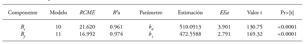
The first fitting indicated that the models are suitable for estimating B _S , B _b , B _f and B _t ; although with heteroscedasticity problems (Figure 1).

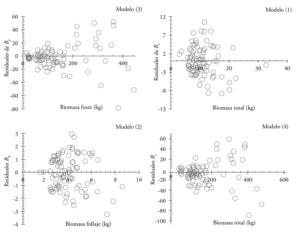
Figure 1 Residual distribution from models used to estimate the biomass of each structural component and the total in Eucalyptus urophylla at Huimanguillo, Tabasco, Mexico. 

Correction by heteroscedasticity and models fitted with seemingly unrelated regressions (SUR) technique (Table 4) ensured the homogeneous distribution of the residuals in the variance of the constant errors (Figure 2). The first system of equations of biomass (SI) was constructed with the correction and new adjustment of the models.

Table 4 Goodness of fit and parameter estimates of the biomass models for clonal trees of Eucalyptus urophylla in Huimanguillo, Tabasco, Mexico 

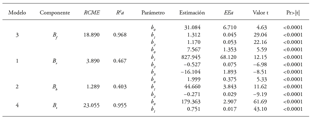
B _S , B _b , B _f and B _t : Bole, branches, leaves and total biomass, each. RMSE: root mean squared error. R ²a: adjusted coefficient of determination. EEa: approximate standard error of the parameters. t Value: value of the Student t distribution, Pr>| t |: probability associated with the Student t value.

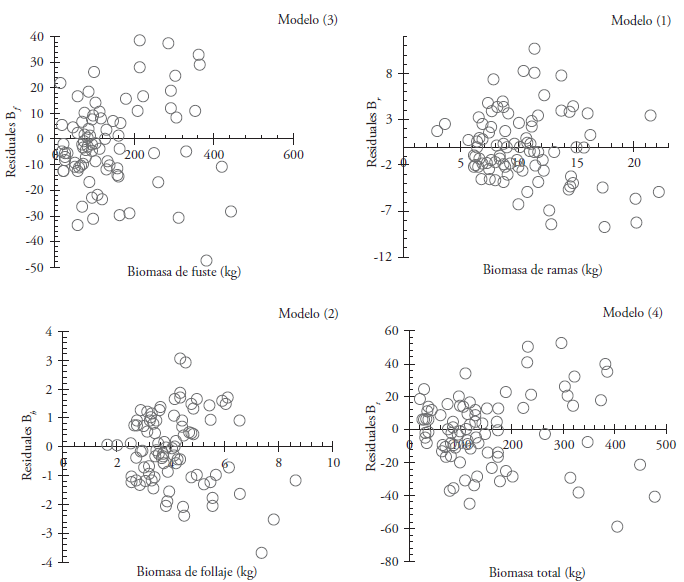
Figure 2 Distribution of residuals corrected for heteroskedasticity of the models used to estimate the biomass by structural and total components in Eucalyptus urophylla at Huimanguillo, Tabasco, Mexico. 

Three structural components and the total biomass in the SW test obtained values between 0.91 and 0.98. These values indicate that there was no normality violation of the regression, in all four cases. The result is similar to those reported by ^{Balzarini et al. (2008)} and applied by ^{Gaillard et al. (2014)}.

Model 5, adjusted with the “backward” and “forward” regression procedures and variables selection, allowed to identify more appropriate models by including additional variables, which with greater precision explain the biomass prediction of branches and foliage:

(15)

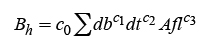(16)

These models were simultaneously fitted and corrected for heteroskedasticity with the power function (Figure 3); the latter gave rise to a second system of equations (SII) were used for the stem (3), total (4), and branches and foliage (15 and 16) biomass estimation. This system had a greater statistical fit (Table 5), which makes it statistically more reliable. The SW test showed the normality of the data with values between 0.91 and 0.97 for the four adjusted models.

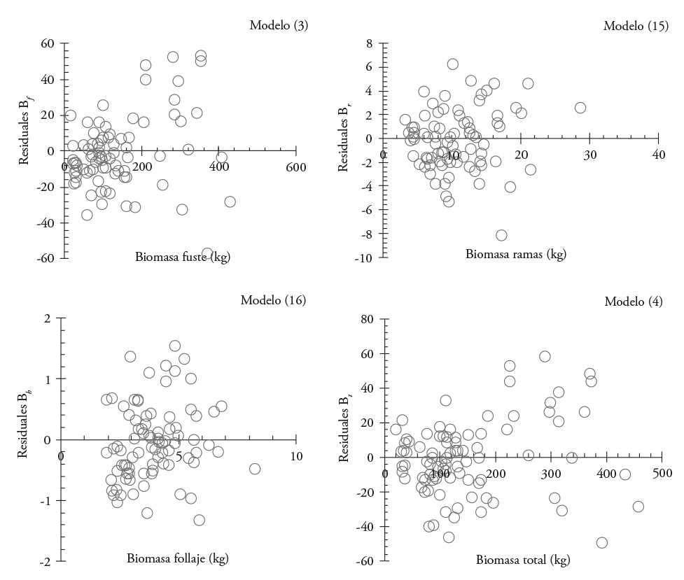
Figure 3 Distribution of residuals when corrected for heteroskedasticity the best-fitted models to estimate biomass by structural component in Eucalyptus urophylla at Huimanguillo, Tabasco, Mexico. 

Table 5 Parameters estimates and goodness of fit statistics to include the height of clean bole and summation variables of the basal diameters of branches by structural component biomass for Eucalyptus urophylla in Huimanguillo, Tabasco, Mexico. 

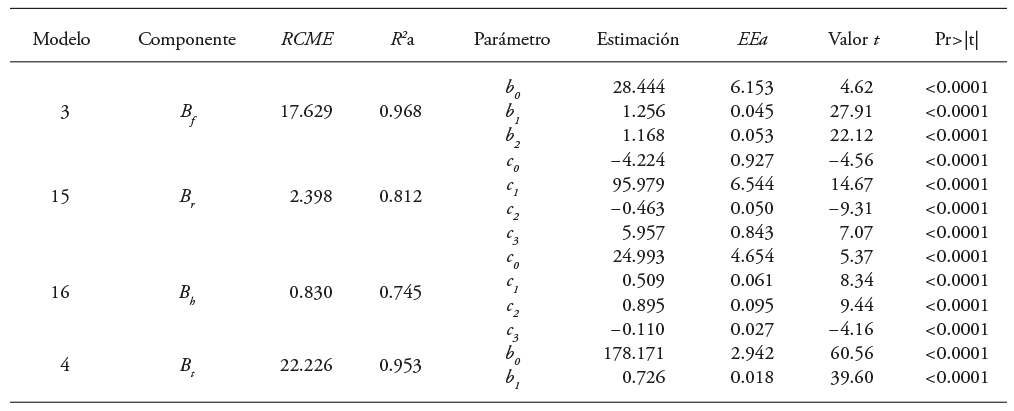
B _S , B _b , B _f and B _t : bole, branches, leaves and total biomass, each. SMER: root mean squared error. R ²a: adjusted coefficient of determination. EEa: approximate standard error.

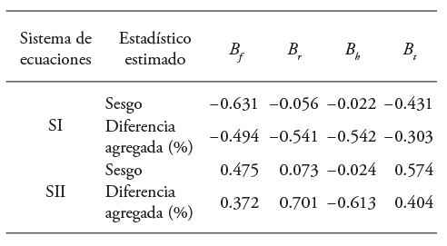
According to the results, although the parameter values of the selected models were close, SII slightly overestimated B _s , B _b and B _t . The B _f estimation was conservative in the prediction per individual and the total difference per sample. The first system (SI) according to the value of the precision statistics underestimated all the variables and made conservative biomass aerial calculations (Table 6).

Table 6 Evaluation statistics of the predictive capabilities of total biomass and by component of equation systems for Eucalyptus urophylla at Huimanguillo, Tabasco, Mexico. 

Due to the accuracy of the adjustment statistics of the equation systems (SI and SII), since they were generated to estimate the total aerial biomass and its components, without using destructive methods, the total biomass and by components can be estimated with information of traditional forest inventory or with additional variables. These can be obtained through electronic measuring instruments such as the dendrometer (Criterium RD 1000®).

Biomass expansion factors (BEF)

The average BEF obtained with equations 6 and 7 showed that 17 % of the aerial biomass distributes in branches and foliage. The rest (83 %) is in the bole (Table 7). This distribution agrees with ^{Téllez et al. (2008)} of E. urophylla plantations in Oaxaca, Mexico, which reported 17.6 % biomass of branches and foliage, and 82.4 % in the trunk. The results from ^{Álvarez-González et al. (2005)} with E. globulus, in Spain, had 14.1 % of leaves and branches biomass, and 85.9 % of trunk, and results of ^{Ferrere et al. (2008)} in Argentina, showed the biomass distribution in E. viminalis with 20 % in branches and foliage and 80 % in trunk.

Table 7 Biomass expansion factors (BEF) by diametric category for aerial biomass data. 

Estimates with systems I and II underestimated 1.51 % and 1.48 % BEF. SII had better approximate evaluated values by diameter class, without considering the age of the plantation.

When considering age in the analysis, the SI, on average, had better approximations but underestimated the BEF by 2.5 %. In this case, we proposed that 19 % of biomass corresponded to branches and foliage, and 81 % to the trunk. This situation is similar to the biomass proportions by structural component (Table 8). In both systems, the BEF for E. urophylla total aerial biomass decreased as the total area increased (^{Rodríguez-Ortiz et al., 2012}; ^{Chávez-Pascual et al., 2013}).

Table 8 Biomass expansion factors (BEF) by age, for aerial biomass data. 

With model 8 for BEF, for B _t , the average total biomass per m³ of timber volume was 600.94 kg. In this case, the factor decreases with the increase of the trees dimensions. For the diameter classes of 10 and 15 cm there were on average 795.05 kg m^-3, for 20 and 25 cm it was 557.94 kg m^-3, and for 30 cm and 35 cm, it was 447.82 kg m^-3. The results for age indicate that the average for these plantations, with 1 to 7 years, was 652.22 kg m^-3, and exhibit a similar trend from 7 to 4 years of age, with 531.06 kg m^-3, 613.34 kg m^-3 at 3 years and increased to 812.25 kg m^-3 in the 1-year-old plantations. This is due to the large amount of foliar biomass that young plantations have.

In the BEF case for B _s , the averages were of 496.45 kg m^-3 per CD and 503.02 kg m^-3. The results analyzed by CD showed 508.76 kg m^-3, 500.03 kg m^-3 and 480.45 kg m^-3 for plantations with dimensions of 10 and 15 cm, 20 and 25 cm, and 30 and 35 cm, each. In both cases, BEF decreased with tree growth and age increase. This was due to the fact that the biomass accumulation in the stem increases as the individual decreases the aerial leaf biomass, which happens either as the diameter classes or ages increase.

The models (10) and (11) for estimating Bt and Bs that considered the linear relationship of these variables to the volume of the tree (m³) showed a BEF of 510.06 kg m^-3 and 472.54 kg m^-3 (Table 9). These results were similar to those of models 8 and 9.

Table 9 Goodness-of-fit statistics and parameters of models 10 and 11 to estimate Bt and Bs in Eucalyptus urophylla trees in CFP at Huimanguillo, Tabasco, Mexico. 

RMSE: root mean squared error. R ²a: determination coefficient adjusted by the number of parameters. EEa: approximate standard error. b ₀ and b ₁: estimated parameters. t value: Student t distribution value. Pr>|t|: probability associated with the Student t-value.

Comparison of estimation methods and inventory of aerial biomass

The results of the analysis of variance of the means of the observed data versus the three SI and SII estimates and the volume-related direct proportion models (10 and 11) conclude that the variables B _t and B _s were equal to each other (Pr>F=0.963 for B _t and Pr>F=0.997 for B _s ). Therefore, the null hypothesis (H ₀ ) is accepted, and the three proposed methods are statistically equal and reliable to estimate these variables. They only differ in the mathematical structure of the models.

In a comparison of the results, taking as reference the bole biomass and total biomass of models 3 and 4 of the first system of equations, showed that the model 12 for volume is the most suitable to estimate the aerial biomass with inventory data, followed by model 13 and model 14 (Table 10). The analysis of variance between the estimates, with the t-Cramer test show that they are equal to each other because the probability value in the ANOVA test was high (F=2.6887 and p=0.7978).

Table 10 Simple random sampling estimates for Eucalyptus urophylla CFP between one and seven years old established at Huimanguillo, Tabasco, Mexico with models 10 and 11. 

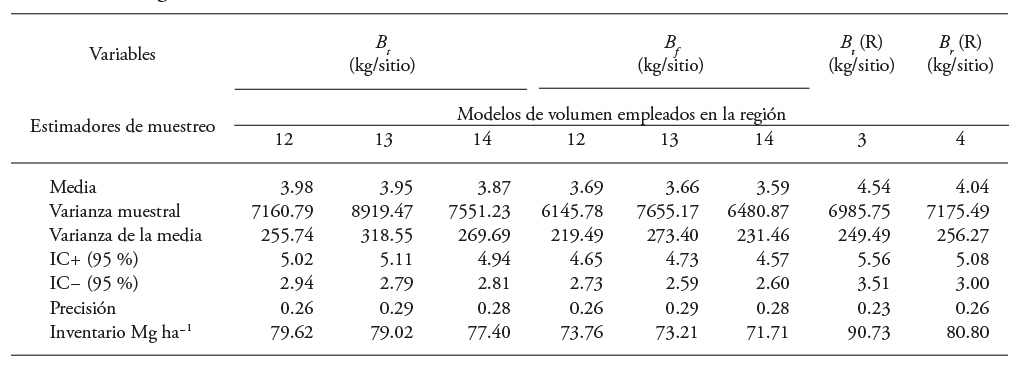
B _f , B _r , B _h y B _t : bole, branches, leaves and total biomass, each. R: value of the reference biomass. IC+: upper limit of the 95 % confidence interval, IC-: lower limit of the confidence interval.

The inventory data analyzed with simple random sampling statistics indicated an average of 156.08 m³ ha^-1 volume in CFPs of E. urophylla, 14 cm in normal diameter, 18 m height and 986 trees ha^-1 density. In addition, incorporating the results in Table 10 in the B _t model 4 (m³ ha^-1), the estimated volume was of 80.80 Mg ha^-1 of aerial biomass. This is consistent with the 70.27 Mg ha^-1 of 7-year-old E. viminalis plantations at Argentina (^{Ferrere et al., 2008}). However, the value is lower than the reported yield in 5, 6 and 7 years old plantations of E. nitens (yield of 73.1, 111.8 and 159.5 Mg ha^-1), with planting density of 1,500 trees per hectare, before (^{Geldres et al., 2006}).

The aerial biomass per hectare was similar to the yield (142 Mg ha^-1) estimated in plantations of E. globulus in Spain. Because the amount reported in this study is on average, half of the reported at 13 years old plantations by ^{Álvarez-González et al. (2005)}. In addition, these estimates, according to the scenarios proposed by ^{Seppánen (2002} and ²⁰⁰³⁾ for E. urophylla, E. grandis and the E. grandis x E. urophylla hybrid are low. because at age 7 it is expected to have an average aerial biomass yield of 147.7 Mg ha^-1 in this region, in the less favorable scenario.