Greenhouse crop mathematical models

Mathematical crop models simulate characteristics such as growth through several plant physiological processes, for example, photosynthesis, respiration, transpiration and crop development. These models can put to test different hypotheses on crop performance without the need to conduct experiments, thus reducing costs. Good approximations can be obtained with mathematical crop models when they are suitably calibrated and evaluated (^{Bouman et al., 1994}, ^{Wallach et al., 2006}).

Studies on application of models to greenhouse crops have been developed in The Netherlands where dynamic models based on biological processes have also been developed. Initially, these studies were developed in numerical form using principles of biological balances, evaluated against experimental data, and finally applied in crop systems (^{Van Straten et al., 2011}).

For tomato, several growth models have been developed over the years, some very simple and others very complex. A deterministic greenhouse tomato growth model written in Pascal language was developed based on a model of leaf assimilation plus a theory of respiration and another of the range of photosynthesis, which is controlled by environmental conditions and carbohydrate contents in the leaves. The model was applied to estimate the effect of CO₂ enrichment on tomato fruit production (^{Kano and Van Bavel, 1988}). For dry matter distribution among plant leaves, stem, root and fruits, ^{Heuvelink and Marcelis (1989)} developed a dynamic model. Their results of simulation of dry matter among tomato leaves, stems and fruits corresponded reasonably well with measured experimental data.

The TOMGRO model for tomatoes, which integrates the Acock model, was used to calculate net crop photosynthesis. The results show that the model is inadequate for describing the CO₂ balance of a greenhouse agrosystem. However, it was determined that it can be used in a more complex model to describe tomato growth and development (^{Zekki et al., 1999}).

There are other models for tomatoes under greenhouse conditions. One of them is TOMPOUSSE, which predicts production of tomato crops (^{Abreu and Meneses, 2000}). Moreover, ^{Dai et al. (2006)} developed a relatively simple model for prediction of biomass production of the canopy as well as for harvested fruits for three greenhouse crops, including tomatoes. The results show that the model satisfactorily predicts canopy biomass and fruit harvest for the three crops. Furthermore, ^{Dimokas et al. (2008)} proposed a new model modified from the original TOMGRO model. The model was evaluated and calibrated in greenhouse tomato and a good relation between measured and simulated data were found for crop development and for biomass and fruit production. This experiment was conducted in Mediterranean conditions in eastern Greece.

Optimal control in greenhouses

Optimal control methods allow obtaining trajectories of environmental conditions inside the greenhouse, which would lead to achieving previously established production goals. These methods are based on a dynamic model that describes the desired crop behavior and establishes an optimization criterion (^{Bryson and Ho, 1975}; ^{Lewis, 1986}). For this reason, development of optimal controls in greenhouses is a topic that recently has been very actively studied. Below, we give a brief description of these studies, which are alternatives to the method we propose.

The work of ^{Boaventura Cunha et al. (1997)} and ^{Coelho et al. (2005)} present a general technique of predictive control to regulate greenhouse environmental conditions. This technique predicts future states of the system when an optimal control trajectory is obtained at a fixed time horizon and recalculated for each time horizon. ^{Tap et al. (1996}, ¹⁹⁹⁷⁾ propose an algorithm of optimal control that is applied at certain time horizons called RHOC (Receding Horizon Optimal Control) and evaluated during the reproductive stages of tomato production. The objective of our study was to obtain the suboptimal temperature trajectory required to maximize production of tomato (Solanum lycopersicum L.) fruit weight (W _F ) and harvested fruit (W _F ) using the Monte Carlo method. The hypothesis was that, by using numerical simulations, it is possible to determine the suboptimal temperature trajectory on which the greenhouse should be maintained for a period of 120 dat in order to increase tomato production.

Dynamic tomato model under greenhouse conditions

Types of mathematical models are empirical, explanatory and teleonomic. It is the explanatory type that is of interest to our study. Explanatory models are defined through a set of ordinary differential equations that describe the behavior of the system state variables, that is, those variables that represent the relevant properties or attributes of the system under consideration (^{López-Cruz et al., 2005}).

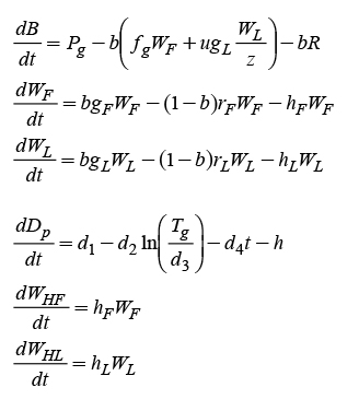
The mathematical model used in our study was proposed by ^{Tap et al. (1996)} and consists of six dynamic equations and, consequently, six state variables, which are described here:

(1)

B[gm^-2] represents the accumulation of assimilates of dry matter per unit of plant area. That is, the metabolic resources that allow the plant to carry out all of its biological processes. W _F [gm^-2] and W _L [gm^-2] are dry weight of fruit and leaves still on the plant. D _p [adimensional] is a parameter that indicates the stage of plant development on a zero to one scale, while W _HF [gm^-2] and W _HL [gm^-2] represent, respectively, harvested fruits and leaves, that is, those that were detached from the plant.

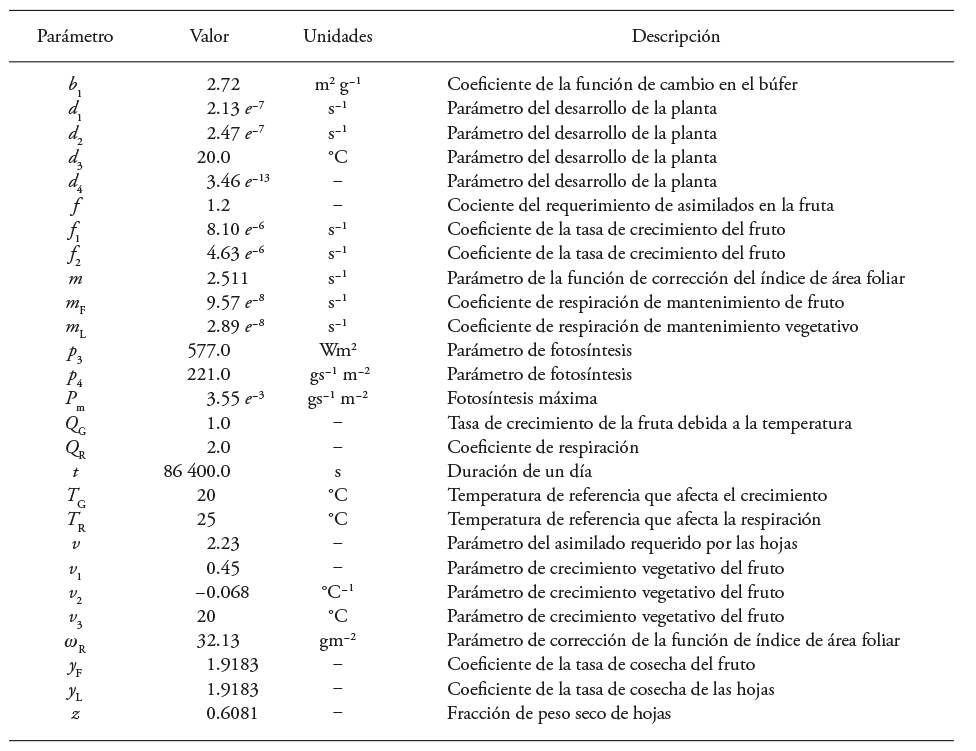
The model described by ^{Tap et al. (1996)} was evaluated by ^{Juárez-Maldonado et al. (2012)} in two tomato crop cycles in a chapel-type greenhouse covered with polycarbonate for two climatic conditions in Saltillo, Coahuila, Mexico (25°25’36” N, 100°59’44” O). Because of the model’s evaluation and calibration process, its parameters (^{Juárez-Maldonado et al. (2012)} were different from those of ^{Tap et al. (1996)}. The modified parameters in our study (Table 1) were used in the dynamic model (1) with which the problem of greenhouse tomato production maximization was determined and solved by manipulating the temperature.

Table 1 Description of the parameters of (1) obtained from ^{Juárez-Maldonado et al. (2012)}. 

Dynamic optimization

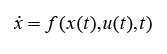
The dynamic system to be studied is the following:

(2)

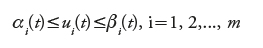
where x(t) ϵ R ⁿ is the state, f(x(t), u(t), t) represents a vector of non-linear functions described in system (1), that is, all the functions in vector form on the right of the equation, and u(t) ϵ R ^m is the vector of control inputs, which are delimited as follows:

(3)

where α _i (t), β _i (t) are known functions. Moreover, we have the vector of initial conditions defined as

(4)

The interval of interest is [0, t _f ] , where t _f is the final defined time. The problem consists of finding the entries for the control u(t) in an interval of time [0, t _f ] that would lead the system to the trajectory x(t), t ϵ [0, t _f ] so that a function or variable is maximized in the entire time interval from [0, t _f ]. In our case, this function is known as the cost function and is given in the following form:

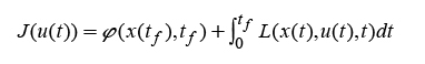(5)

where L is the Lagrangian of the system that contains its dynamic evolution expressed in equation (1) (^{Van Straten et al., 2011}) and φ(x(t _f ), t _f ) is a final condition that can be imposed on the system.

In this study, the dynamic greenhouse tomato growth model developed by ^{Tap et al. (1996)} was the basis for calculating a suboptimal temperature trajectory that would maximize fruit (W _F ) and harvested fruit (W _HF ) production of greenhouse tomatoes. To solve this problem, the Monte Carlo random solution method was selected. This method establishes a temperature range and aims to determine the configuration that guarantees a maximum value for tomato fruit (W _F ) and harvested tomato fruit (W _HF ) weight. Temperature was selected as the parameter to calculate because of its greater effect on plant development and growth and because it is one of the factors in which many resources are invested for its control. The Monte Carlo method was selected also because it is possible to obtain approximations of results without knowing the system’s behavior since it is necessary only to give value entries and determine which value has the greatest probability of occurring and generating the desired system behavior.

The first step is to determine the trajectory of the control entries u(t) that the greenhouse should maintain during a period of 0 to 120 dat and during tomato development to increase production, using numerical simulations of model (1) with the parameters of Table 1 and application of the Monte Carlo method. The assumption is that by using numerical simulations, it is possible to determine the suboptimal trajectory of the control entries u(t) that would increase tomato production. To achieve this, maximizing fruit weight (W _F )and harvested fruit weight (W _HF )are posed considering two cost functions, which are described below:

In the first, only maximum growth of the variable W _F was considered in a time interval of [0,120] dat and manipulating the control inputs u(t), that is:

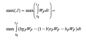(6)

subject to the following restrictions: u ^min ≤u(t) ≤u ^max and that the dynamic equations of system (1) are satisfied.

In the second, maximization of both fruit weight (W _F ) and harvested fruit weight (W _HF ) were considered. In this way, from the initial time up to harvest time, 0 to 58 days after transplant, the goal was only to maximize productivity of W _F , and finally, from harvest (59 dat) up to the final growth period (120 dat) W _HF was increased; that is,

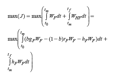(7)

Likewise, subjected to the restrictions of the previous case, the goal was not to obtain a maximum value of only W _HF from the beginning of the simulation since this variable remains constant with a value of zero until the harvest stage is reached. To achieve this objective, one or several inputs of the dynamic system (1) must be selected, such as temperature, PAR radiation, or CO₂ concentration.

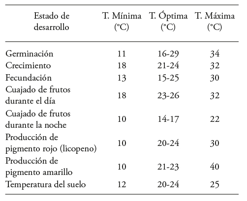
Temperature is one of the main climatic factors that affect development stages and physiological processes of the plant. This can be seen in the dynamic model (4) as T _g , which is one of its inputs. Satisfactory development of the phases of germination, vegetative growth, flowering, fruit set and fruit ripening depend on the temperatures inside the greenhouse at each growth stage. Moreover, because tomato is a plant that is sensitive to extreme temperature and/or changes in relative humidity, it is necessary to maintain it within an optimum temperature range so that it can achieve its maximum development. Also, it should be added that tomato is a thermoperiodic plant, which means that its growth is favored by temperature that varies with the stage of plant development, as can be seen in Table 2 (^{Jaramillo-Noreña et al., 2013}; ^{Wallach et al., 2006}).

Table 2 Minimum, maximum and optimal temperatures for plant development stages reported by ^{Jaramillo-Noreña et al. (2013)} and ^{Wallach et al. (2006)}. 

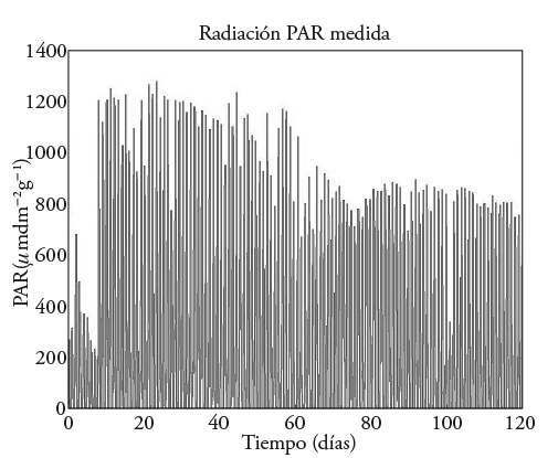
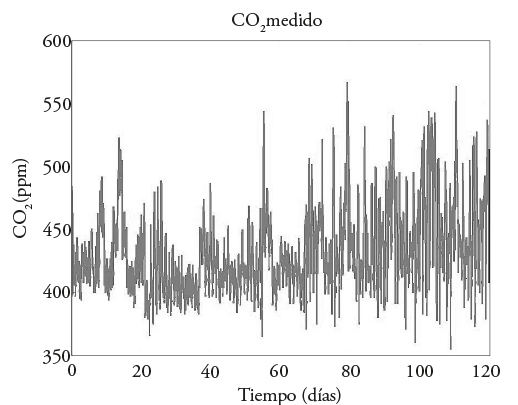
Thus, to achieve the objective of maximizing production based on dynamic model (4), temperature is selected as the control input (Table 2) to obtain, first, a temperature trajectory that maximizes the quantity of fruit on the plant during the period of 120 dat. Another temperature trajectory is then chosen to maximize the quantity of fruit in the first 58 dat and harvested fruit from day 59 to 120 dat. It is important to clarify two points. First, despite the existence of another two inputs in dynamic model (1), which correspond to PAR (I) radiation and CO₂ concentration, these were not determined in our study; rather, we used those reported by ^{Juárez Maldonado et al., 2012} (Figures 8 and 9). Second, to obtain a feasible temperature trajectory in maximizing tomato production, in either of the two problems posed here, it is necessary to have a restriction on temperature, which is the manipulated input. For this reason and considering the studies of ^{Pérez et al. (2002)}, ^{Jaramillo-Noreña et al. (2013)} and ^{Wallach et al. (2006)}, a temperature restriction interval of 15 °C≤T _g ≤30 °C was chosen. This range was selected since it is the mean temperature range during the day in the city of Saltillo.

The problem of maximizing fruit is formulated with the system of differential equations (1), which describes the growth dynamics of cultivated tomato plants. Considering the control input u=T _g , which is restricted to the range of 15 °C≤u≤30 °C, that is, u [15;30] and considering the vector of states, x(t)=[B, W _F , W _L , D _p , W _HF , W _HL ] , with the initial crop conditions of x(0)=[0; 0,42; 43,59; 0; 0; 3,95] obtained by ^{Juárez-Maldonado et al. (2014)}, it is necessary to find the temperature trajectory that generates a higher quantity of fruit (W _F ) and of harvested fruit (W _HF ) in the final growth period t _{f =} 120 days. It is important to mention that each time interval in which a temperature is calculated is 15 min during the 120 d of simulation.

The Monte Carlo Method

The Monte Carlo method consists of generating random numbers on the basis of a given probability distribution. In this way, configurations, or inputs, accessible for the system are explored to later take those of greater probability based on selected criteria.

The algorithm based on the Monte Carlo Method (^{Peña Sánchez de Rivera, 2001}) used to obtain the temperature trajectory is the following:

One step of Monte Carlo is considered completed when the entire process described above has been carried out. The suboptimal temperature trajectory is obtained by calculating the averages of T _g in the iterations done to graph them against the established time intervals using the equation of the mean, Tg= 1M∑I=1M Tg1 where T _gi is the temperature obtained in step i of the simulation and M is the total number of iterations.

Because it is random and not based on the conditions of first and second order optimality (^{Bryson and Ho, 1975}; ^{Lewis, 1986}), the Monte Carlo method must be evaluated by changing the number of iterations. It is known that, by increasing the number of iterations, the method can better approximate its solution. Therefore, it depends on the finalization criterion when determining the maximum error to be admitted. For this reason, to solve the previous problem, two simulations are carried out: one with 500 thousand and the second with 1 million iterations with the Monte Carlo method for the two cases of maximizing the variables fruit weight (W _F ) and harvested fruit weight (W _HF ), considering that the temperature limits are between 15 and 30 °C.

First case: maximization of W _F

The suboptimal temperature trajectories obtained after day 59 for the first case of only W _F maximization, which corresponds to 1 million iterations, indicates that temperature stabilizes around 15 °C, the lower limit of the imposed restriction, unlike what occurs at 500 thousand iterations where no stabilization is observed. Moreover, it can be observed that the suboptimal temperature trajectory shows periods that emulate day and night around this same restriction interval (Figure 1).

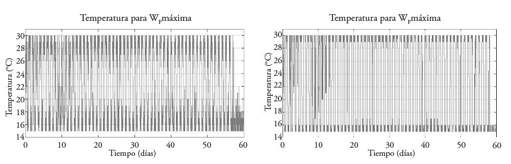
Figure 1 Suboptimal temperature trajectories when maximizing W _F . obtained with 500 thousand iterations (left) and with 1 million iterations (right). 

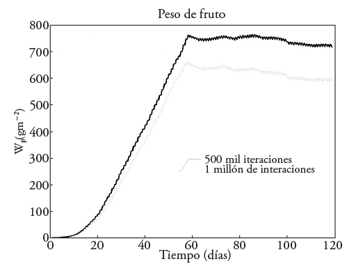
Maximized fruit weight (W _F ) with the suboptimal temperature trajectory (Figure 1), for 500 thousand and 1 million iterations, reveals that the increase in the number of iterations has an impact on obtaining maximized fruit weight and that, for 500 thousand iterations, around 650 [gm^-2] W _F is obtained, while for the case of 1 million iterations, 750 [gm^-2] W _F is obtained (Figure 2).

Figure 2 Maximized W _F [gm^-2] obtained with 500 thousand iterations and with 1 million iterations. 

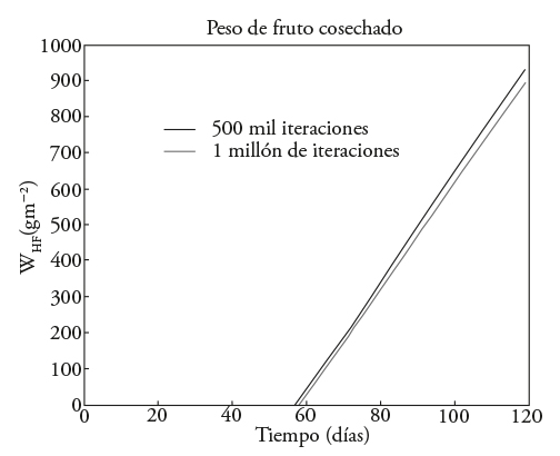
The results of harvested fruit (W _HF ), when only fruit weight (W _F ) is maximized considering 500 thousand and 1 million iterations, indicate that the curve begins to increase around day 59, which is when fruit harvest initiates. Harvested fruit weight (W _HF ) reaches an approximate value of 900 [gm⁻²] for both 500 thousand iterations and for 1 million iterations (Figure 3).

Figure 3 W _HF [gm^-2] obtained with 500 thousand iterations and with 1 million iterations. 

Second case: maximization of W _F and W _HF

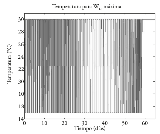
The suboptimal temperature trajectory obtained for combined maximization of W _F and W _HF , shows a periodicity similar to that when only fruit weight W _F is maximized. However, as of day 59, approximately, corresponding to the harvest stage, maximization indicates that temperature should be maintained at around the upper limit of temperature restriction of 30 °C (Figure 4).

Figura 4 Trayectorias de temperatura subóptima para W_F y W_HF. Obtenida con 500 mil iteraciones (izquierda) y con 1 millón de iteraciones (derecha). 

The results of fruit weight (W _F ) indicate values similar to the first case in the period of 0-59 d, 650 [gm^-2] and 750 [gm^-2] W _F for 500 thousand and 1 million iterations, respectively. However, as of day 59, both simulations of fruit weight (W _F ) decrease since in this case only harvested fruit weight is maximized (W _HF ) (Figure 5).

Figure 5 Maximized W _F [gm^-2] obtained with 500 thousand and with 1 million iterations. 

Harvested fruit weight (W_HF) increases considerably, relative to the case in which only fruit weight (W _F) is maximized; that is approximately 1300 [gm^-2] and 1450 [gm^-2] are obtained for 500 thousand and one million iterations, respectively, contrasting with the 900 [gm^-2] obtained previously (Figure 3).

Results of the simulation without the optimization reported by ^{Juárez-Maldonado et al., (2012)}

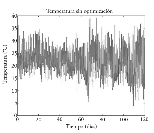
The results of fruit weight and of harvested fruit weight reported by ^{Juárez-Maldonado et al. (2012}), reproduced by simulation and presented here (Figure 7), maximize neither W_F nor W _HF. Only the trajectories of temperature, CO₂ and PAR radiation, measured during the 120 dat in the greenhouse were considered (Figures 8-10). These results show an increase in fruit weight (W _F ) of 600 [gm^-2] without maximization to 750 [gm^-2] when maximizing only W _F with 1 million iterations (Figure 2). In comparison, when harvested fruit weight (W _HF ) is maximized, as of day 59 there is an increase of 800 [gm^-2] without maximizing to 1450 [gm^-2] (Figures 7 and 6). The temperatures recorded in the study of ^{Juárez-Maldonado et al. (2012)}, without optimization (Figure 8), compared with the suboptimal trajectories reported in Figures 2 and 4, change greatly. A production cost analysis to compare crop development without control and with temperature trajectory suboptimization is necessary before deciding whether its application is possible.

Figure 6 Maximized W_HF [gm^-2] obtained with 500 thousand iterations and with 1 million iterations. 

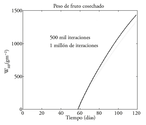
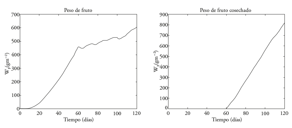
Figure 7 Fruit weight (left) and harvested fruit (right) reported by ^{Juárez-Maldonado et al. (2012)}. 

Figure 8 PAR radiation reported by ^{Juárez-Maldonado et al. (2012)}. 

Figure 9 CO₂ concentration reported by ^{Juárez-Maldonado et al. (2012)}. 

Figure 10 Temperature reported by ^{Juárez-Maldonado et al. (2012)}. 

The results revealed two important characteristics. The first is approximation of the solution when the number of iterations of the Monte Carlo method is increased from 500 thousand to 1 million. Considering this variation in iterations, less oscillation is observed in the graphs (Figures 1 and 4) with a larger number of iterations. This is expected since, as steps increase, the system tends to convergence of the solution to the problem (^{Peña Sánchez de Rivera, 2001}). The second is the behavior of the temperature trajectory for maximization of only fruit weight (W _F ), for W _F maximization between days 0 and 58 and for harvested fruit weight (W _HF ) from day 58 to the end of the period (120 d). From day 59, which marks the beginning of harvest, the suboptimal temperature trajectory stabilizes around 15 °C for maximization of W _F (Figure 1) and around 30 °C for maximization of W _F and W _HF (Figura 4). The latter behavior can be explained by the dynamics of W _F and W _HF (eq. 4): dWFdt= bgFWF-1-brFWF dWHFdt= hFWF . It can be observed that both are linked by the term h _F W _F , and in the case of W _F , production shrinks, while for W _HF , the same term allows an increase in harvested fruit. Also, it can be seen that the suboptimal temperature trajectory for both cases shows periods that emulate day and night, around this same restriction interval before day 59.

Optimal temperature

To obtain the optimal temperature trajectory, the Monte Carlo method with 1 million iterations was compared with application of optimal control using MATLABR11 (^{MathWorks, 2017}) with the non-linear optimization tool and DYNOPT software based on the study of ^{Logsdon and Biegler (1989)}, and an optimal control trajectory was determined given a dynamic model of a process, which is subject to restrictions of equality and inequality. Because of limited space, we show only the optimal temperature trajectory in the case of W _F and W _HF maximization (Figure 11), which is similar to that shown in Figure 4. The difference is due to the random nature of the Monte Carlo method in which temperature tends to oscillate around the mean, or expected, value, and this oscillation is directly related to the number of simulation steps, while in the non-linear optimization method, these oscillations do not exist.

Figure 11 Optimal temperature trajectory calculated with DYNOPT optimal control software.