


Services on Demand
Journal
Article
 text in
  English (pdf)
 Article in xml format
 Article references
 Send this article by e-mail
Indicators
-
 Cited by SciELO
 -
 Access statistics
Related links
-
 Similars in
SciELO
Similars in
SciELO
Share

 Permalink
Agrociencia
On-line version ISSN 2521-9766Print version ISSN 1405-3195
Agrociencia vol.51 n.3 Texcoco Apr./May. 2017
Water-Soils-Climate
Calibration of the usle and musle soil loss models in a mexican forest watershed: El Malacate case study
1Posgrado de Ingeniería Agrícola y Uso Integral del Agua. Universidad Autónoma Chapingo. Carretera México-Texcoco. Km. 38.5, Chapingo, Texcoco, Edo. de México. 56230. (mauricio@correo.chapingo.mx), (mara2883@hotmail.com).
2Instituto Mexicano de Tecnología del Agua. Paseo Cuauhnáhuac 8532, Jiutepec, Morelos, 62550. México. (privera@tlaloc.imta.mx, prr.imta@gmail.com).
3CONAGUA. Estado de Zacatecas, Zacatecas, México. (felipe.deleon@conagua.gob.mx)
The quantification of water erosion in watershed soils serves to understand their degree of deterioration and to implement conservation measures that minimize the loss of soil. Given the lack of information to quantify soil erosion in México with acceptable precision, it is necessary to study their estimation with the information available through methodologies validated with experimental information. For that purpose, the objective of this study was to calibrate the USLE (Universal Soil Loss Equation) and MUSLE (Modified USLE) methods in the El Malacate micro-basin, which belongs to the Pátzcuaro Lake watershed in Michoacán, México, with experimental data from 2013. The MUSLE model was calibrated satisfactorily through the adjustment of the K factor whose value was 0.1067. Prior to the calibration the errors in the estimation of the results were -214.1 and -721.6 %, using the value of the K factor that results from the original methodology proposed by Wischmeier-Smith, and from the proposal updated by FAO. According to the delivery rate from soil to the exit of a watershed, reported in other studies for watersheds similar to that of the study, it was found that the USLE model does not represent the characteristics of the El Malacate basin. Instead, the calibrated MUSLE model can be used to estimate the sediment yield in watersheds with similar conditions with scarce hydrometric and precipitation information. Given that the K, C, LS and P factors are common in both models, the methodology should be reviewed to obtain the R factor and the mathematical structure of their representation in the MUSLE model, in addition to the methodologies used to calculate the delivery rate for the soil and the C and K factors, to guarantee the compatibility of their results.
Key words: Specific degradation; soil erosion; sediment production; hydrological modelling; simulation in watersheds
La cuantificación de la erosión hídrica de los suelos en cuencas hidrográficas sirve para conocer el grado de su deterioro y para implementar medidas de conservación que minimicen la pérdida del suelo. Dada la carencia de la información para cuantificar con precisión aceptable la erosión en México, es necesario estudiar su estimación con la información disponible mediante metodologías validadas con información experimental. Por tal motivo, el objetivo de este estudio fue calibrar los modelos USLE (EUPS o Ecuación Universal de la Pérdida del Suelo, por sus siglas en inglés) y MUSLE (EUPS modificada) en la microcuenca El Malacate, perteneciente a la cuenca del Lago de Pátzcuaro en Michoacán, México con información experimental de 2013. El modelo MUSLE se calibró satisfactoriamente mediante el ajuste del factor K cuyo valor fue 0.1067. Previo a la calibración los errores en la estimación de los resultados fueron -214.1 y -721.6 %, usando el valor del factor K resultante con la metodología original propuesta por Wischmeier-Smith, y con la propuesta actualizada por la FAO. De acuerdo con la tasa de entrega de suelo a la salida de una de cuenca, reportada en otras investigaciones para cuencas similares a la de nuestro estudio, se encontró que el modelo USLE no representa las características de la cuenca El Malacate. En cambio, el modelo calibrado MUSLE puede utilizarse para estimar la producción de sedimentos en cuencas de condiciones similares con escasa información hidrométrica y de precipitación. Dado que en ambos modelos son comunes los factores K, C, LS y P, se debe revisar la metodología para obtener el factor R y la estructura matemática de su representación en el modelo MUSLE, además de las metodologías para calcular la tasa de entrega de suelo y los factores C y K, para garantizar la compatibilidad de sus resultados.
Palabras clave: Degradación específica; erosión del suelo; modelación hidrológica; producción de sedimentos; simulación en cuencas
Introduction
México has grave soil losses caused by water erosion. The Ministry of the Environment and Natural Resources (Secretaria de Medio Ambiente y Recursos Naturales, SEMARNAT, 2008), based on a study carried out by the Universidad Autónoma Chapingo in 2003, informed of a potential water erosion of 42 % of the national surface. It also reported water erosion by then of 22.73 million ha, of which 56.4 % was at a low erosion level (5 to 10 Mg ha-1 year-1), 39.7 % in a moderate situation (10 to 50 Mg ha-1 year-1) and 3.9 % in the grave category (more than 50 Mg ha-1 year-1). These specific potential degradations imply that a large part of the national territory would surpass the maximum advisable limits of soil loss established in the USA agricultural manual (Wischmeier and Smith, 1978) and FAO’s (CP, 1991).
The potential erosion values must be taken only as reference values, since the erosion process is quite complex and its adequate representation depends on information about it, and of the precise estimation of the characteristics of the study site (Sadeghi et al., 2014; Kinell, 2015). The precise quantification of water erosion of the soils in hydrographic watersheds serves to establish the conservation measures to be implemented to minimize the loss of the soil resource (Wischmeier and Smith, 1978). With this purpose, studies have been performed regarding the production of sediments in basins in many parts of the world, using different methodologies. For example, in experimental plots of a few square meters up to huge watersheds covering hundreds of square kilometers, a specific global average degradation of 1.9 Mg ha-1 year-1 was observed, with a maximum of 64 in China and a minimum of 0.00005 in Canada (De Araújo and Knight, 2005).
In order to estimate the production of sediments at the exit of a basin, three types of models are used: 1) empirical, such as USLE and MUSLE, based on simple functional relations resulting from experimental observations (Williams, 1975; Wischmeier and Smith, 1978; Renard et al., 1997); 2) based on processes with strong empirical support, such as those developed with neuronal networks (Heng and Suetsugi, 2013; Garg, 2015); and 3) physical, based on conservation principles such as EUROSEM and KINEROS (Morgan et al., 1998; Rosenmund et al., 2005).
The models based on physical principles and in processes demand much information, although obtaining it is complicated. Because of this, the USLE and MUSLE models are used individually (Sadeghi et al., 2014) or integrated into more complex models such as SWAT to quantify the transport of sediments (Ayana et al., 2012; Prabhanjan et al., 2015). The mathematical structure of these models is simple and their use would be simple due to the existence of tables, nomograms and reference equations to calculate their components (factors) in manuals and publications, originated in the USA (Wischmeier and Smith, 1978; Renard et al., 1997; NEH, 2004), and in some cases adapted to the conditions of other countries (Figueroa et al., 1991; Pongsai et al. 2010). However, studies performed in Asia (Sadeghi et al., 2007; Pongsai et al. 2010), Africa (Muche et al., 2013), South America (Guevara-Pérez and Márquez, 2007; Besteiro and Gaspari, 2012), and Europe (Rosenmund et al., 2005) show that the models require adjustments.
In México, the USLE and MUSLE models are also used as reference to quantify the erosion of soils, although, in their majority, the results are estimatives because they were not validated with experimental data (Flores et al., 2003), or they were compared with little field information, without specifying or arguing the adjusted factors (Torres et al., 2005). Some experiments were developed in the state of Michoacán and that of Ajuno stands out (Tapia et al., 2002), a site that belongs to the Pátzcuaro Lake watershed, and the basin of the Cointzio Dam (Bravo et al., 2009b). However, because they are experimental plots with specific crops and treatments, their results are not valid to represent the behavior of a watershed as a single unit of hydrologic response, since only one portion of the soil detached from the surface reaches the exit of a watershed and sediment yield is the result, in addition to sheet and rill erosion represented by the USLE and MUSLE models, from the erosion that takes place in gullies, streambed, streambanks, road banks and mass landslides (NEH, 1983). In this regard, the MUSLE model can represent adequately the sediment yield at the exit of a watershed, for its factors can be integrated into the erosion process and the soil transport (Sadeghi et al., 2007; Arekhi et al., 2012).
In this context it is neccesary to study the predictive efficiency of the estimation models for sediment yield in México’s watersheds, with the aim of having a support tool for decision making for a sustainable management. Therefore, the objective of this study was to calibrate the USLE and MUSLE models in the El Malacate forest micro-basin, located in the Pátzcuaro Lake watershed based on a broad set of experimental information obtained during 2013, of daily precipitation, hydrographs, and amount of solids in suspension in the runoff events, images supervised of use of soil and vegetation, content of organic matter in the soil, and texture and soil structure. In particular, the results would serve as reference to estimate the production of sediments in neighboring watersheds, with similar conditions to those of the study, to implement measures that stop the soil deterioration in the Pátzcuaro watershed, because the erosion rates exceed the permissible limits (Huerto and Vargas, 2014).
Materials and Methods
Description of the study place
This research was carried out in the El Malacate micro-basin with an extension of 149.2 ha. The micro-basin is part of the Pátzcuaro Lake closed watershed, municipality of Tzintzuntzan, state of Michoacán de Ocampo, with a mean altitude of 2300 m, between 19° 36’ 50’’ and 19° 38’ 30’’ N, and 101° 35’ 10’’ and 101° 36’ 20’’ W. According to the Köppen climate classification, modified by García (2004), the climate in the area is temperate sub-humid C (w2) with annual mean temperature between 12 °C and 18 °C, temperature of the coldest month between -3 °C and 18 °C, and temperature of the warmest month between 20°C and 30°C, and an annual precipitation of 200 to 1800 mm with a mean value of 920.3 mm (IMTA, 2009).
Experimental data
The cartographic information used was the digital elevation model (DEM), map of soil and vegetation uses, and map of the type of soil by INEGI at a scale of 1:50 000. The map of land and vegetation uses was verified in the field where a predominance of forest use was identified. To verify the type of soil, a visit was carried out along the watershed, and the type of soil nitic Luvisol was found, based on the FAO-UNESCO classification, made up of four layers, with a superficial layer of 25 cm of loam clay sand texture (32.5 of clay, 51.3 of loam, and 6.09 % of very fine sand), and fine granular structure with 4.98 % of organic matter.
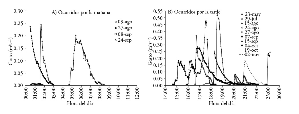
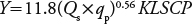
The daily precipitation in 2013 was recorded, appraised at intervals of 0.2 mm with a HOBO RG3-M pluviograph, with an annual total of 769.6 mm. The hydrographs were also used (Figure 1), as well as the amount of sediments at the exit of the basin, obtained from 14 runoff events recorded in 2013. The hydrographs were obtained through a long-throated flume with an ultrasonic sensor to measure the water depth, and an automatized system to record the information. The sediment production was obtained by quantifying the amount of solids in suspension from samples taken at the exit of the basin during the runoffs.
Estimation models in the production of sediments
USLE Model The Universal Soil Loss Equation (USLE) was proposed to compute longtime average soil losses from sheet and rill erosion under specified conditions (Wischmeier and Smith, 1978), and is defined as:
 (1)
(1)
where, according to the international metric system of units (Foster et al. 1981), A is the annual erosion rate per unit of area (Mg ha-1 year-1), R is the rainfall and runoff erosivity factor (MJ mm ha-1 h-1 year-1), K is the soil erodibility factor (Mg ha-1 MJ-1 mm-1), L is the slope length factor (dimensionless), S is slope steepness factor (dimensionless), C is the cropping management factor (dimensionless), and P is the support practice factor (dimensionless).
MUSLE model
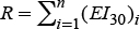
The MUSLE model (Williams, 1975) is a modification of the USLE model, and it consists in replacing the R factor of erosivity of the rain because of superficial runoff and the peak runoff rate of a storm, with the aim of calculating the sediment yield per event and expressed as:
 (2)
(2)
where Y is the sediment yield in a specific event (Mg event-1), Qs is the runoff volume (m3) and qp is the peak runoff rate of the event (m3 s-1).
Calculation of the factors from USLE and MUSLE
The runoff volumes and the peak runoff rate were obtained from the hydrographs measured. The average values of the K, R, LS, C and P factors were calculated. The P erosion control practice factor was considered equal to the unit because conservation practices were not performed. The K factor was calculated by employing a single type of soil with the information reported in the experimental data, the R factor was obtained with data from rain, and the LS and C factors were obtained in a weighted form by the area (Sadeghi et al., 2007; Pongsai et al., 2010), through the processing of MED and the map of land and vegetation uses with ArcGis version 10.1, whose procedures for calculation are described next.
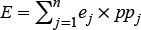
R factor
This factor represents the potential capacity that rain drops have to cause erosion and it was calculated in two ways: through the EI30 index (Wischmeier and Smith, 1978), and with an equation adapted by Figueroa et al. (1991), who consider a quadratic functional relationship with the mean annual precipitation registered.
The EI30 method was used because there is daily information about precipitation, registered at intervals of minutes. This method is defined as the product of the total kinetic energy of a rain event by the maximum intensity in 30 min, so that the total value of the factor of the rain erosivity R is the sum of values of erosivity of individual storms, calculated as follows: (Wischmeier and Smith, 1978):
 (3)
(3)
where E is the kinetic energy of the rain from each storm (MJ ha-1 mm-1), I30 is the maximum intensity of rain in any 30 min from each storm (mm h-1), and n is the number of storms in the year.
The kinetic energy of each storm is the eddition of the kinetic energies of the rain intervals, differentiated by their rain intensities, and it was calculated with the equation proposed by Wischmeier and Smith (1978):
 (4)
(4)
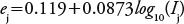 (5)
(5)
where ej is the kinetic energy of the interval of rain j of a storm (MJ ha-1 mm-1), and Ij is the intensity of the rain from interval j (mm h-1), and ppj is the precipitation of the interval j (mm). For intensities greater than 76 mm h-1 an e value of 0.283 was established.
According to the criterion to calculate EI30 proposed by Wischmeier and Smith (1978), the storms with precipitations lower than 12.5 mm with rain periods separated more than 6 h were not considered, unless 6.2 mm or more had fallen in 15 min (I15≥24.8 mm h-1). The existence of rain periods in long storms was defined when the sheet was less than 1.2 mm in a lapse of 6 h (Renard et al., 1997).
The R factor is calculated with the equation adapted by Figueroa et al. (1991) as a methodological alternative to the watersheds where it is not possible to calculate the EI30 for lack of detailed information from the precipitation throughout the year. The watershed of study is located in the hydrological zone V (Bravo et al., 2009a), with the following equation:
 (6)
(6)
where P is the annual precipitation of 2013 in millimeters.
K factor
The term erodibility of the soil is used to indicate the susceptibility of a soil to erosion. It is defined as the rate of soil loss for each additional unit of EI30 when the slope and its length, the plant cover, and the conservation practices of the soil remain constant and its values are equal to one (Wischmeier and Smith, 1978).
As the sum of the loam particles plus the very fine sand was less than 70 % of the total of soil particles, the K factor was calculated with the equation proposed by Wischmeier and Smith (1978):
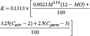 (7)
(7)
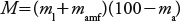
where M is a parameter of the particle size, MO is the percentage of organic matter (%), C estr is a code of soil structure, Cperm is a code of soil permeability, and 0.313 is a conversion factor of the system of English units to the international metric system (Foster et al, 1981). The parameter of the particle size was calculated as:
 (8)
(8)
where ml is the percentage of loam content (diameter of particles of 0.002 to 0.05 mm), mamf is the percentage of the content of very fine sand (diameter of 0.05 to 0.10 mm), and ma is the percentage of the content of clay (diameter of particles smaller than 0.002 mm).
The value of the soil permeability was determined in function of their texture using the functional relations described by Saxton and Rawls (2006).
Another method was that of FAO (1980), which is used in México, since the K factor is determined only in function of the unit to which the soil belongs in the FAO-UNESCO classification and of the texture of the superficial layer.
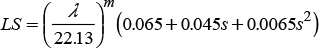
LS factor
This factor represents the effect of the topography on soil erosion. The erosion increases as the length (L) of the plot increases in the direction of the slope, and the inclination of the surface (S) increases, calculated as (Wischmeier and Smith, 1978):
 (9)
(9)
where:
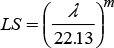 (10)
(10)
 (11)
(11)
where λ is the plot slope length (m), s is the slope of the plot (%), and the m exponent of the factor of the slope length considers the proportion of erosion caused by the erosion between drains, due to the impact of the drops, and that caused in drains by the dragging force of the flow (Renard et al., 1997). The value of m varies in function of the slope of the plot and was calculated with the equation proposed by McCool (Renard et al., 1997):
 (12)
(12)
where θ is the angle of slope.
The classical equation to calculate the LS factor, proposed by Wischmeier and Smith (1978), does not represent well the effect of the topography on the soil erosion for slopes greater than 16 % (Pongsai et al., 2010), so that the S factor was calculated with the equation proposed by McCool (Renard et al., 1997) for slopes greater than 9 %:
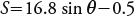 (13)
(13)
where θ is the angle of the slope.
C factor
The C Factor of crop management and soil cover is the relationship of losses in a plot cultivated under specific conditions, with regards to the losses of naked soil and with continuous fallow under the same conditions of soil, slope and rain (Wischmeier and Smith, 1978).
For its calculation, the methodology and values proposed by Wischmeier and Smith (1978) were used. In rainfed agriculture, where maize is sown predominantly, it was quantified through the erosivity indexes EI30 in each one of the stages of cultivation and the relative soil losses in cultivation areas compared to lands under continuous fallow.
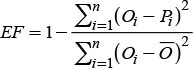
Evaluation of the model’s adjustment
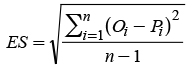
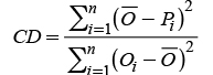
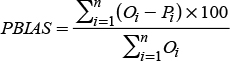
The correspondence between the series of values observed and those estimated are expressed in terms of four indexes: Model’s efficiency (EF) proposed by Nash and Sutcliffe (1971) and used by Besteiro and Gaspari (2012), and Muche et al. (2013); standard error (ES) (Pongsai et al. (2010); coefficient of determination (CD) (Rosenmund et al., 2005); and percentage of bias (PBIAS) (Moriasi et al., 2007). The equations of the indicators are given by:
 (14)
(14)
 (15)
(15)
 (16)
(16)
 (17)
(17)
where Oi are the values observed, Pi are the values predicted, Ō is the average of the values observed, and n is the number of data evaluated.
The model increases the precision of the prediction of the values observed as the values of the indicators EF, ES, CD and PBIAS approach one, zero, one, and zero, respectively.
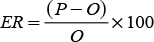
The correspondence between the pairs of data observed and estimated was made through the relative estimation error, calculated as (Pongsai et al., 2010; Arekhi et al., 2012):
 (18)
(18)
The optimal value of ER is zero; positive values indicate the percentage of over-estimating of the model, while negative values quantify the percentage of sub-estimating of the model.
Results and Discussion
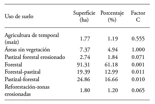
The value of the K factor was 0.034 with Equation (7) proposed by Wischmeier and Smith (1978), and 0.013 with the methodology proposed by FAO. The values of the LS, C (Table 1) and P factors were 10.1, 0.062 and 1.0, respectively.
Table 1 Values of the C factor according to the land and plant use in the El Malacate watershed, Michoacán.
The value of the R factor calculated with Equation (6), proposed by Figueroa et al. (1991) and calculated with an annual precipitation of 769.6 mm, was 2163.2 MJ mm ha-1 h-1.
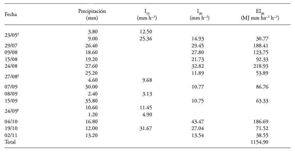
The value of the R factor calculated with the erosivity indexes, considering only the storms when there were runoffs and which fulfilled the criteria of Wischmeier and Smith (1978), was 1154.9 MJ mm ha-1 h-1 year-1 (Table 2). This result corresponded to the sum of rain events with precipitated sheets greater than 12.5 mm or with sheets lower than 12.5 mm, but with rain intensities above 24.8 mm h-1 in any 15 min (I15). The storms of September 8 and 24 produced sediment dragging but they were not considered because they did not comply with the criteria established, since precipitations of less than 12.5 mm took place and I15 lower than 24.8 mm h-1. In the storms of May 23 and August 27, there were two rain periods, and only one of them fulfilled the requirements to be taken into account in the EI30.
Table 2 Erosivity index EI30 of the storms with runoff events in 2013.
There were two rain periods in the storm.
Calibration of the MUSLE model
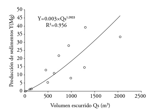
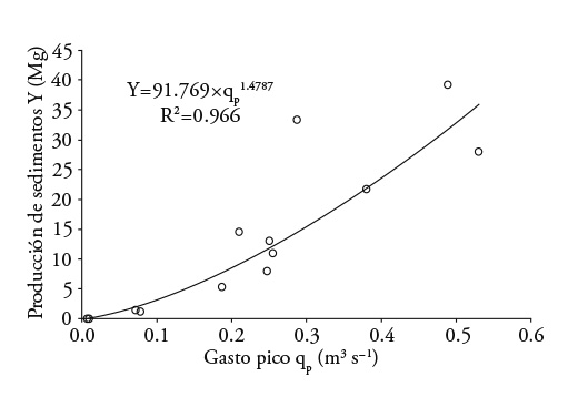
Figures 2 and 3 show a potential relationship between the production of sediments and the runoff volumes and peak runoff rate of each storm, as Williams (1975) points out. The adjustment of these relationships was R2>0.95, but the standard deviations were high; when relating the sediment production with the runoff volume, the standard error was 8.2 and 6.6 Mg when it depended on the peak expenditure, as Sadeghi et al. (2007) reported.
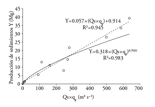
When relating the production of sediments with the product of the runoff volume by the peak runoff rate, term by which Williams (1975) substituted the erosivity factor of R rain of the USLE, there is good adjustment in a potential-type model (R2=0.983; Figure 4). However, the value of the power (0.703) is higher than the one found by Williams (1975) in the US (0.56), and the standard error was 4.4 Mg. A model of linear type also presented an adjustment R2=0.945 with a lower standard error to the potential type (3.1 Mg), but with the disadvantage of not representing the phenomenon for products Qsxqp close to zero (Figure 4).
The errors made by the potential relationship between the sediment production and the product Qs xqp, added to the estimation errors of the K, LS and C factors, led to strong errors between the values observed and predicted by the MUSLE model. In fact, the results from Table 3 and the statistical indicators of columns 3 and 4 from Table 4 show the need for adjustment of the factors from the MUSLE model.
Table 3 Relative errors in the estimation of sediment production with the MUSLE model.
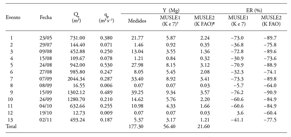
† The K factor was calculated with Equation (7). ¶ The K factor was calculated with the FAO methodology.
According to the total results from sediment production (Table 3), it was found that the MUSLE1 model (K factor calculated with Equation 7) underestimated the results in 12 of the 13 rain events, and the MUSLE 2 model (K factor calculated with the methodology by FAO) underestimated the results in all the events. The results have the tendencies reported by Sadeghi et al. (2007), who found underestimations by the MUSLE model for short-lasting small storms. This is explained because the MUSLE model was developed for grassland watersheds with larger storms and slopes smaller than those of the watershed in study (Williams, 1975).
Both MUSLE models underestimated the results, but it is notable that the FAO model is less precise and the relative estimation error calculated with Equation (18) for the annual data reported in Table 3 was -68.2 %, while with the other model it was -87.8 %. These results imply that the FAO model did not represent adequately the K factor and it is more advisable to use Equation (7) because, in addition to considering the soil texture, it considers the structure, permeability and organic matter content.
For the calibration of the model, only one of the factors is adjusted and it tends to be the one for which there is little information, or in which the conditions of the site of study are not contemplated in the tables, nomograms and equations suggested in publications about the subject. This is indicated by Pongsai et al. (2010), Besteiro and Gaspari (2012) and Sadeghi et al. (2014).
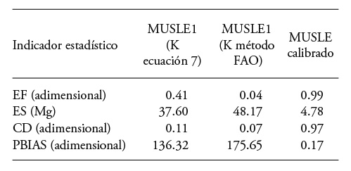
Since the P factor is well-defined with a value of one because there are no management practices, the topography changes very little in time; the characteristics of the land and vegetation uses remain similar throughout the year because it is a watershed that is mostly forest and the growth of plant species is slow. In our study, we set out to adjust the K factor due to the dynamic behavior of the soil, which during the year acquires different degrees of humidity and vulnerability to erosion (Kinell, 2015). Proof of the difficulty to represent the value of the K factor is the great difference in the estimations between the model that included the K value calculated with Equation (7), and the one obtained with the FAO method.
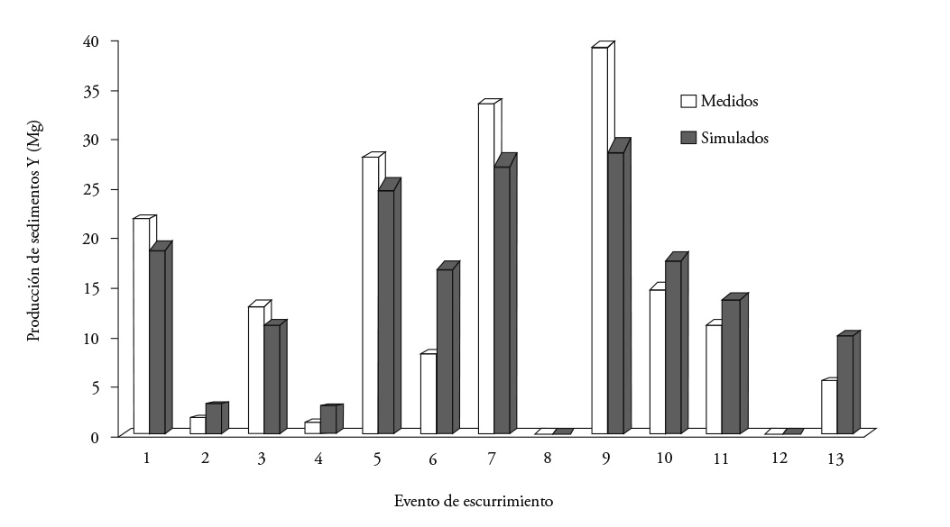
The value of the calibrated K factor was 0.107 and was obtained through the technique of least squares regression. In México there are no experimental values of K from similar watersheds for their comparison. In micro-basins of the Pátzcuaro Lake watershed and other neighboring ones, studies were performed in runoff plots of some crops with different types of farming, but in most of the cases the calibrated factor corresponds to crop C (Tapia et al., 2002; Bravo et al., 2009b) and it is assumed that the other factors of the USLE model are the correct ones and calculated with the methodology proposed by Wischmeier and Smith (1978). Table 4 shows that the values of three (EF, CD and PBIAS) of the four statistical indicators of adjustment are quite close to their optimums. The value next to the unit of the Nash and Sutcliffe (EF) indicator establishes that the calibrated model is efficient. The ES value implies that there was a standard error of 4.78 Mg in the production of sediments and given the 149.2 ha of the watershed, it translates into a standard error of 0.03 Mg ha-1. The CD value next to the unit indicates that the values predicted suggested the trend of those measured, compensating the errors; thus, in some events the results were overestimated and in others underestimated (Figure 5). The final balance resulted in an average underestimation of 0.17 Mg (PBIAS).
The calibrated MUSLE model can be used to estimate in an approximate way the production of sediments in other watersheds of similar conditions to those of our study, and where there are no gauge data as observed by Prabhanjan et al. (2015) with the application of the SWAT module, which is supported by the MUSLE model (Ayana et al., 2012). There are similar basins, as is verified in the results obtained in a discharge basin into the Tzurumútaro drainage in the state of Michoacán, also mostly forest, and the production of sediments was 0.8 Mg ha-1 year-1 from 2007 to 2010 (Huerto and Vargas, 2014), which is similar to the 1.2 Mg ha-1 year-1 measured in the micro-basin of our study.
Calibration of the USLE model
For the review of the USLE model results, the values of the K, LS, C and P factors of the calibrated MUSLE model were taken up again, and the measured value of the R factor, since the MUSLE model predicts the soil erosion better (Muche et al., 2013). In the methodology established by Wischmeier and Smith (1978) and in the revision of the USLE model by Renard et al. (1997), it is not specified clearly whether the criterion to calculate the EI30erosivity index must be applied only for the storms where there are runoffs or for all the storms; it is also not specified whether the erosivity of storms that do not satisfy such a criterion for the calculation of EI30 but which did produce runoffs should be contemplated.
If the EI30 of the storms with presence of runoffs from Table 2 (1154.9) and without the presence of runoffs (992.1) are considered, resulting from adding the values outside the parentheses of Table 5, the total annual value in 2013 was 2147.0 MJ mm ha-1 h-1, quite near to the value of 2163.2 obtained with Equation (7), proposed by Figueroa et al. (1991). The good representation of the R factor of the estimative method is evident for the year of study, with an error of 0.75 % with regards to the total measure of events with or without runoffs (2147.0 MJ mm ha-1 h-1). However, if the mean annual precipitation of 920.3 mm (IMTA, 2009) is used to calculate R, according to Figueroa et al. (1991) instead of using the one recorded in 2013, the R value is 2464.7 MJ mm ha-1 h-1 and higher than 14.8 % to the measured one (2147.0 MJ mm ha-1 h-1).
Table 5 Monthy values of EI30 (MJ mm ha-1 h-1) from storms without runoffs.

The numbers between parentheses indicate the of the month when the event took place.
According to the magnitude of the production of sediments in some storms that did not fulfill the criteria for the inclusion of the EI30 in the R factor, it is necessary to consider the storms where there were runoffs and sediment production, even when they do not comply with the requirements fixed, as it happened in the event of September 24th when there were two rain periods (Table 2), and the sediment production in that storm was significant (14.6 Mg) compared to the production of the other runoff events (Table 3). Similarly, in the runoff event on May 23rd, with considerable sediment production (21.8 Mg) (Table 3), the erosivity index was not considered in one of the two rain periods (Table 2). In addition to this event, there were no storms immediately before as possible influence, since the nearest one took place on May 14th with a precipitation of 1 mm in 2.7 h.
With values of 10.1, 0.062 and 1.0, respectively, for the LS, C and P factors, the calibrated value of K (0.1067) for the MUSLE model, and the measured value of R (2147) used, the USLE model resulted in an erosion rate of 143.0 Mg ha-1 year-1. The sediment production at the exit of a basin ranges from 33 to 100 % of soil losses, from sheet and rill erosion, represented by the USLE model, in the US (NEH, 1983; Calhoun and Fletcher III, 1999). For the analysis of the result, if it is considered that the sediment production in the study basin was due only from sheet and rill erosion, and it is assumed that 37 % of its value reached the discharge point of the watershed obtained from the national engineering manual from the US (NEH, 1983) in function of the area of the micro-basin, a sediment production of 52.9 Mg ha-1 year-1 would be expected, which is higher than the one measured in the study basin (1.2 Mg ha-1 year-1) and even the one observed in basins with high erosion rates such as Las Huertitas, which discharges 15 Mg ha-1 year-1 to the Cointzio Dam in the state of Michoacán (Duvert et al., 2010).
The USLE model estimates the average annual soil loss of many years in the terrain, and, an erosion of 3.25 Mg ha-1 year-1 would need to take place in order to satisfy the soil delivery rate to the watershed’s exit of 37 % (1.2 Mg ha-1 year-1). Pero this amount represents large variability compared to the 143.0 Mg ha-1 year-1 estimated for the year 2013, and implies that for some years there would need to be much higher erosion than this value. These results show that the delivery rate considered does not represent the characteristics of the study basin, and that the cultivation factor considered was not the adequate one.
The results from the USLE model suggest the benefit of adapting the methodologies used for: 1) obtaining the R factor, and the shape of its representation through the Qsxqp product in the MUSLE model, since the value of the power of this term (0.7031) was higher than the 0.56 proposed by Williams (1975), as is shown in the potential functional relation in Figure 4; 2) calculating the factor of the crop C and the soil K; and, 3) calculating the delivery rate to the basin’s exit where the contributions of sediments from erosion in gullies, streambed, streambanks, roadbanks and mass landslides would need to be considered (NEH, 1983; Calhoun and Fletcher III, 1999). This adaptation would allow a compatibility of results between the USLE and MUSLE models, when applied to the study basin.
Conclusions
The MUSLE model was calibrated for 2013 through the adjustment of least squares of the K factor with values of the indicators of the statistical adjustments next to the optimums. Prior to the calibration, better results were obtained when using the K value calculated with Equation (7) proposed by Wischmeier and Smith, instead of the one obtained with the FAO methodology. The model could be used to estimate the sediment production in watersheds from similar conditions to those of El Malacate, Michoacán, for which there is little hydrometric information that is detailed.
The USLE model did not represent the loss of erosion that took place in the study watershed and we suggest revising the methodologies to calculate the delivery rate to the basin’s exit, and the C, R and K factors.
The values of the R factor calculated with the compared equations were similar, if all the rain events in the year are considered. However, their meaning and the methodology to calculate them with the USLE model and its equivalence in the MUSLE model must be revised, since the slope of the runoff volume product from peak runoff rate was higher compared to that suggested by Williams (1975)
Literatura Citada
Ayana, A.B., D.C. Edossa, and E. Kositsakulchai. 2012. Simulation of sediment yield using SWAT model in FinchaWatershed, Ethiopia. Kasetsart J. (Nat. Sci.) 46: 283-297. [ Links ]
Arekhi, S., A. Shabani, and G. Rostamizad. 2012. Application of the modified universal soil loss equation (MUSLE) in prediction of sediment yield (Case study: Kengir Watershed, Iran). Arab. J. Geosci. 5:1259-1267. [ Links ]
Besteiro, S. I., y F. J. Gaspari. 2012. Modelización de la emisión de sedimentos en una cuenca con forestaciones del noreste Pampeano. Rev. FCA UNCUYO 44: 111-127. [ Links ]
Bravo E., M., M.E. Mendoza, y L. Medina O. 2009a. Escenarios de erosión bajo diferentes manejos agrícolas en la cuenca del lago de Zirahuén, Michoacán, México. Inv. Geogr., Boletín 68: 73-84. [ Links ]
Bravo E., M., M. E. Mendoza, L. Medina O., C. Prat, F. García O., and E. López G. 2009b. Runoff, soil loss, and nutrient depletion under traditional and alternative cropping systems in the transmexican volcanic belt, central Mexico. Land Degrad. Dev. 20:640-653. [ Links ]
Calhoun, R. S., and C. H. Fletcher III. 1999. Measured and predicted sediment yield from a subtropical, heavy rainfall, steep-sided river basin: Hanalei, Kauai, Hawaiian Islands. Geomorphology 30: 213-226. [ Links ]
CP (Colegio de Postgraduados). 1991. Manual de conservación del suelo y del agua: Instructivo. Tercera edición. CP. Chapingo, México. pp:3-6. [ Links ]
De Araújo, J. C., and D.W. Knight. 2005. A review of the measurement of sediment yield in different scales. R. Esc. Minas, Ouro Preto 58: 257-265. [ Links ]
Duvert, C., N. Gratiot, O. Evrard, O. Navratil, J. Némery, C. Prat, and M. Esteves. 2010. Drivers of erosion and suspended sediment transport in three headwater catchments of the Mexican Central Highlands. Geomorphology 123: 243-256. [ Links ]
FAO (Organización de las Naciones Unidas para la Alimentación y la Agricultura). 1980. Metodología provisional para la Evaluación de la Degradación de los Suelos. Roma, Italia. 86 p. [ Links ]
Figueroa S., B., A. Amante O., H. G. Cortes T., J. Pimentel L., E. S. Osuna C., J. M. Rodríguez O., y F. J. Morales F. 1991. Manual de Predicción de Pérdidas de Suelo por Erosión. SARH-Colegio de Posgraduados. Salinas, San Luis Potosí, México.150 p. [ Links ]
Flores L., H. E., M. Martínez M., J. L. Oropeza M., E. Mejía S., y R. Carrillo G. 2003. Integración de la EUPS a un SIG para estimar la erosión hídrica del suelo en una cuenca hidrográfica de Tepatitlán, Jalisco, México. Terra 21: 233-244. [ Links ]
Foster, G. R., D. K. McCool, K. G. Renard, and W. C. Moldenhauer. 1981. Conversion of the universal soil loss equation to SI metric units. J. Soil Water Cons. 36: 355-359. [ Links ]
García, E. 2004. Modificaciones al Sistema de Clasificación Climática de Koppen. Quinta edición. Instituto de Geografía. UNAM. México, D.F. 220 p. [ Links ]
Garg, V. 2015. Inductive group method of data handling neural network approach to model basin sediment yield. J. Hydrol. Eng. 20: C6014002. [ Links ]
Guevara-Pérez, E., and A. M. Márquez. 2007. Comparison of three models to predict anual sediment yield in caroni river basin, Venezuela. JUEE 1: 10-17. [ Links ]
Heng, S., and T. Suetsugi. 2013. Using artificial neural network to estimate sediment load in ungauged catchments of the Tonle Sap river basin, Cambodia. JWARP 5: 111-123. [ Links ]
Huerto D., R. I., y S. Vargas V. 2014. Estudio Ecosistémico del Lago de Pátzcuaro: Aportes en Gestión Ambiental para el Fomento del Desarrollo Sustentable. Volumen II. IMTA, Jitupec, Morelos, México. 204 p. [ Links ]
IMTA (Instituto Mexicano de Tecnología del Agua). 2009. Extractor rápido de información climatológica ERIC III 2.0. IMTA. Jiutepec, Morelos, México. [ Links ]
Kinell, P. I. A. 2015. Geographic variation of USLE/RUSLE erosivity and erodibility factors. J. Hydrol. Eng. 20: C4014012. [ Links ]
Morgan, R. P. C., J. N. Quinton, R. E. Smith, G. Govers, J. W. A. Poesen, K. Auerswald, G. Chisci, D. Torri, and M. E. Styczen. 1998. The European soil erosion model (EUROSEM): a dynamic approach for predicting sediment transport from fields and small catchments. Earth Surf. Process. Landforms 23: 527-544. [ Links ]
Moriasi, D. N., J. G. Arnold, M. W. Van Liew, R. L. Bingner, R. D. Harmel, and T. L. Veith. 2007. Model evaluation guidelines for systematic quantification of accuracy in watershed simulations. Trans. ASABE 50: 885−900. [ Links ]
Muche, H., M. Temesgen, and F. Yimer. 2013. Soil loss prediction using USLE and MUSLE under conservation tillage integrated with ‘fanya juus’ in Choke Mountain, Ethiopia. Int. J. Agric. Sci. 3: 046-052. [ Links ]
Nash, J. E., and J. V. Sutcliffe. 1971. River flow forecasting through conceptual models. J. Hydrol. 13: 297-324. [ Links ]
NEH (National Engineering Handbook). 1983. Chapter 6: Sediment sources, yields and delivery ratios. In: United States Department of Agriculture. National Engineering Handbook, part 632 (Second edition). U.S. Department of Agriculture, SCS. Washington, D.C. http://www.nrcs.usda.gov/wps/portal/nrcs/detail/mi/technical/engineering/?cid=nrcs141p2_024573 . (Consulta: Marzo 2015). [ Links ]
United States Department of Agriculture. 2004. National Engineering Handbook, part 630. Chapter 10: Estimation of direct runoff from Storm Rainfall. U.S. Department of Agriculture, NRCS. Washington, D.C. http://www.nrcs.usda.gov/wps/portal/nrcs/detail/mi/technical/engineering/?cid=nrcs141p2_024573 . (Consulta: Marzo 2015). [ Links ]
Pongsai, S., D. S. Vogt, R. P. Shrestha, R. S. Clemente, and A. Eiumnoh. 2010. Calibration and validation of the modified universal soil loss equation for estimating sediment yield on sloping plots: A case study in Khun Satan catchment of northern Thailand. Can. J. Soil Sci. 90: 585-596. [ Links ]
Prabhanjan, A., E. P. Rao, and T. I. Eldho. 2015. Application of SWAT model and geospatial techniques for sediment-yield modeling in ungauged watersheds. J. Hydrol. Eng. 20: C6014005. [ Links ]
Renard, K. G., G. R. Foster, G. A. Weesies, D. K. McCool, and D. C. Yoder. 1997. Agriculture Handbook 703: Predicting Soil Erosion by Water, a Guide for Conservation Planning with the Revised Universal Soil Loss Equation (RUSLE). USDA. ARS. Washington, D.C. 384 p. [ Links ]
Rosenmund, A., R. Confalonieri, P. P. Roggero, M. Toderi, and M. Acutis. 2005. Evaluation of the EUROSEM model for simulating erosion in hilly areas of central Italy. Riv. Ital. Agrometeorol. 2: 15-23. [ Links ]
Sadeghi, S. H., L. Gholami, A. K. Darvishan, and P. Saeidi. 2014. A review of the application of the MUSLE model worldwide. Hydrol. Sci. J., 59: 1-11. [ Links ]
Sadeghi, S.H., T. Mizuyama, and B.G. Vangah. 2007. Conformity of MUSLE estimates and erosion plot data for storm-wise sediment yield estimation. Terr. Atmos. Ocean. Sci., 18:117-128. [ Links ]
Saxton, K. E., and W. J. Rawls. 2006. Soil water characteristic estimates by texture and organic matter for hydrologic solutions. Soil Sci. Soc. Am. J. 70:1569-1578. [ Links ]
SEMARNAT. 2008. Informe de la situación del medio ambiente en México, capítulo 3. Edición 2008. Compendio de Estadísticas. SEMARNAT, México, D.F. pp:111-132. [ Links ]
Tapia V., L. M., M. Tiscareño L., J. Salinas R., M. Velázquez V., A. Vega P., y H. Guillen A. 2002. Respuesta de la cobertura residual del suelo a la erosión hídrica y la sostenibilidad del suelo, en laderas agrícolas. Terra 20: 449-457. [ Links ]
Torres B., E., E. Mejía S., J. Cortés B., E. Palacios V., y A. Exebio G. 2005. Adaptación de un modelo de simulación hidrológica a la cuenca del río Laja, Guanajuato, México. Agrociencia 39: 481-490. [ Links ]
Williams, J. R. 1975. Sediment-yield prediction with universal equation using runoff energy factor. In: U.S. Department of Agriculture, Agricultural Research Service. Present and Prospective Technology for Predicting Sediment Yield and Sources. USDA. ARS-S40. pp: 244-252. [ Links ]
Wischmeier, W. H., and D. D. Smith. 1978. Predicting rainfall erosion losses: a guide to conservation planning. USDA. SEA. Agriculture Handbook 537. Washington, D.C. 58 p. [ Links ]
Received: March 2016; Accepted: July 2016
 Este es un artículo publicado en acceso abierto bajo una licencia Creative Commons
