Introduction

A suitable design of surface irrigation is essential for efficient application of water, and simulation models developed over the recent five decades have become the main tool for predicting water flow and final distribution of moisture along the furrow or border strip during the process of irrigation (^{Bautista and Strelkoff, 2009}). ^{Strelkoff et al. (2009)} pointed out that the most important factor in surface irrigation, and one of the most difficult to quantify, is infiltration. Therefore, its adequate characterization is fundamental in the good performance of surface irrigation. For modeling infiltration it is possible to solve the ^{Richards (1931}) equation of water flow in partially saturated soils. However, the conditions of heterogeneity are a major problem because of the number of parameters required. Traditionally, infiltration is measured at discrete points with double-cylinder infiltrometers or with instruments such as the disc infiltrometer (^{Angulo-Jaramillo et al., 2000}). With these devices, representative measurements of a single point are obtained, in the best of cases, and their spatial variability can be of such magnitude that adequate average values cannot be easily inferred. To estimate suitable parameters for modeling, techniques for instrumenting irrigation tests were implemented, which can be as elaborate as measuring surface profiles of the water during irrigation. The parameters are obtained with inverse modeling methods, with the advance and recession phases in surface irrigation. They are popular because the data are relatively easy to obtain and the results in some sense represent field averages (^{Strelkoff et al., 2009}).

According to ^{Jury et al. (2011}), an effective property is a functional relationship between amounts averaged over a volume and depends on the scale and the model. Unsaturated hydraulic conductivity is an example of an effective property, defined as the quotient of the flow over the potential hydraulic gradient measured on the same scale. This property is monotonous and unique when the volume is selected in a region with homogeneous soil. But this is not guaranteed when the scale increases and the soil is heterogeneous.

The use of effective hydrodynamic properties has been discussed in specialized literature. ^{Zhu and Mohanty (2006}) analyzed optimal schemes to obtain effective hydraulic properties for transitory infiltration. ^{Mesgouez et al. (2014}) evaluated the uncertainty and validation of estimating effective hydrodynamic properties in simulations of dynamic evaporation. ^{Durner et al. (2008}) studied the movement of water at the scale of a lisimeter to analyze the existence and uniqueness of effective hydrodynamic properties in stratified soils by inverse modeling. The validity of using effective hydrodynamic properties, in most cases, depends on the objective or the variables of interest of the modeling. Consideration of homogeneity of porous media will depend, then, on the phenomenon under study. In the case of surface irrigation, it will be important to consider the heterogeneity of the soils over which the advance wave of irrigation water transits from its position of entry in the furrow or border strip to the end.

The general conditions for representing hydrodynamic properties of the soil with effective parameters were analyzed in this study using parameters generated with experimental information obtained by ^{Zataráin et al. (2003}) for a field in Montecillo, State of Mexico. To analyze the spatial variability of the hydrodynamic properties, the ^{Miller and Miller (1956}) theory of similitude in porous media was used to scale infiltration.

^{Zataráin et al. (2003}) point out that, if the mean of saturated hydraulic conductivity is a constant, representation of the advance phase by effective hydrodynamic characteristics is possible for flows that assure the arrival of the advance front to the end of the furrow. The hypothesis of our study was that the use of mean values of soil hydrodynamic properties in surface irrigation is valid under these two conditions. The objective was to analyze them by modeling the advance phase with two procedures of characterization of the spatial variable: one by generating correlated fields of hydraulic conductivity with a method grounded in spectral analysis and conserving the probability distribution and the other by random generation also conserving probability distribution.

Materials and Methods

Analysis of the conditions for modeling the advance phase in surface irrigation in borders was conducted with the hydrological model that results from a simplification of the equations of Barré de Saint-Venant. The law of resistance proposed by ^{Fuentes et al. (2004}) and the hypothesis of contact time of ^{Saucedo et al. (2006}) were used. To describe infiltration, we used the equation of ^{Green and Ampt (1911}), which can be derived from the equation of ^{Richards (1931}), with no loss of generality, according to ^{Parlange et al. (1982}, ¹⁹⁸⁵). The study of spatial variability of infiltration is simplified with ^{Miller and Miller’s (1956}) theory of similar media (self-similar fractal media).

Description of the irrigation

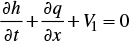
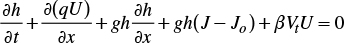
Superficial water flow in border irrigation can be considered unidimensional because of the relationship between the width and depth of the water. With this consideration, irrigation modeling can be done with the Barré de Saint-Venant equations, derived from the principles of mass conservation and the quantity of movement:

(1)

(2)

where x is the spatial coordinate in the main direction of the movement [L]; t is time [T]; q(x, t)=U(x,t)h(x,t) is the flow per unit of width of the border strip, or unitary flow [L²T^-1]; U=U(x,t) is the average flow rate in a cross-section [LT^-1]; h=h(x,t) water depth over the soil surface [L]; J_o=-∂Z/∂x, with Z the vertical coordinate oriented positively upward [L], which is generally assimilated to the topographic slope of the soil surface when the angle of the inclination is small [LL^-1]; J=J(x,t) is the friction slope [LL^-1]; g is gravitational acceleration [LT^-2]; V_I=V_I(x,t)= ∂I(x,t)/ ∂t is the rate of infiltration [LT^-1], I=I(x,t) is the infiltrated volume per unit of width and per unit of length of the border, or infiltrated depth [L]; the adimensional parameter β is defined as β=V_IX/U, where V_IX is the projection in the direction of the movement of the exit rate of the mass of water due to infiltration, which is generally depreciated.

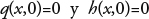
In the advance phase of irrigation, the initial and border conditions are:

(3)

(4)

where q₀ is the constant unitary flow imposed at the entrance of the border strip; x_f (t) is the position of the front of the surge.

To close the system (1)-(4) it is necessary to provide equations for infiltration rate and friction slope with a hydraulic resistance law. To describe infiltration, the ^{Richards (1931}) equation, or a simplification of it, can be used, for example, the ^{Green and Ampt (1911}) model, which is derived from the Richards equation when hydraulic difussivity is assimilated to a Dirac density and non-saturated hydraulic conductivity is continuous (^{Parlange et al., 1982}, ¹⁹⁸⁵).

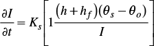
The ^{Green and Ampt (1911}) model is represented by the following differential equation:

(5)

where I is the accumulated infiltrated depth [L]; K_s is saturated hydraulic conductivity [LT^-1]; θ_s and θ_o are moisture content at saturation and initial, respectively, [L³L^-3]; h_f is the suction at the wetting front (piston flow) [L]; h is the depth of water over the soil surface (positive pressure) [L].

The law of hydraulic resistance relates friction slope to average flow rate and water depth. The law proposed by ^{Fuentes et al. (2004}), resulting from the analysis of coupling the equations of Barré de Saint-Venant and Richards, can be used in the singularity present at the entrance of the border strip:

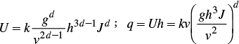(6)

where υ is the kinematic viscosity coefficient [L²T^-1]; k is an adimensional constant that depends mainly on soil roughness; the d potential is such that 1/2<d<1, the lower limit corresponds to the Chézy regime and the upper limit to the Poiseuille regime.

As simplified forms of the Barré de Saint-Venant equations, they identify the diffusive wave, or zero inertia, model wich is obtained from eliminating the inertial terms of equation (2); the kinematic wave model, which results from eliminating the variation in depth in space in the diffusive wave model; and the hydrological model of ^{Lewis and Milne (1938}), which retains the continuity equation and assumes a constant average depth over time and space (h¯). This model also assumes that infiltration depends only on contact time (τ) between water and the soil at a point x, defined by τ(x,t)=t-t_x, where t is the total advance time and t_x is the time it takes for the advance wave to arrive at the point in question.

In a study on surface irrigation Saucedo et al. (2001) used the Barré de Saint-Venant and Richards equations and showed that considering only the infiltrated depth as a function of contact time is sufficient to describe it adequately.

The hydrologic model of Lewis and Milne is an adequate approach in the advance phase of surface irrigation since it conserves its principal characteristics (^{Rendón et al., 1997}; ^{Castanedo et al., 2013}), and it will be retained for the study of spatial variability of hydrodynamic soil properties and their impact on the advance phase because of its simplicity.

The average surface depth can be estimated from the wave profile in steady regime ∂h/∂t=0 and ∂q/∂t=0. From equations (1) and (2), we deduce the following:

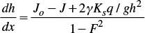(7)

where γ=1-1/2 β; K_s is the steady infiltration flow equal to saturated hydraulic conductivity that can be variable in space [LT^-1] and F is the Froude number: F²=q²/gh³.

Equation (7) is generally integrated numerically, but an approximate analytical solution is obtained if we consider that in the position of the wave front (x=xf), the predominating term is the friction slope: dh/dx≃-J. The friction slope in terms of the depth and flow rate is deduced from equation (6): J=(ʋ²/gh³)(q/kʋ)^1/d

The variation in flow rate, relative to x in steady regime, is obtained from the continuity equation dq/dx+K_s=0 considering the average saturated hydraulic conductivity; that is, q=q₀(1-x/x_max) with x_max=q₀/K_s. Integration leads to h(x)=h_r(1-x/x_max)^δ, with δ=(1+d)/4d and h_r=(v²x_max/δg^1/4, and to extrapolate this profile up to the entrance to the border strip, depth hr is replaced by the normal depth h_o. The average depth is obtained from volume over the area divided by x_max:

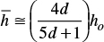(8)

where:

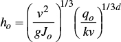(9)

Integration of equation (5) with condition I=0 in t=0, considering constant water depth equal to the average value defined by equation (8), leads to:

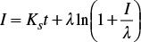(10)

where λ = (h- + hf)(θs-θo)

Equation (10) has h_f and K_s as unknown parameters. θ_s and θ_o can be measured, and ̄h is estimated with equation (8) if the adimensional roughness coefficient is known.

Infiltration and spatial variability

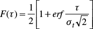
For the analysis of spatial variability of infiltration, the data reported by ^{Zataráin et al. (2003}) were used. The experiments were conducted in a sandy soil in Montecillo, Estado de Mexico. In a 100 m long, 5 m wide border strip with a longitudinal slope of J_o=0.002 mm^-1, 21 infiltration tests were conducted in a transect at the center of the crop bed. The first of these was done at the beginning of the bed and the rest at 5 m, relative to the test just before. The double cylinder method (^{Angulo-Jaramillo et al., 2000}) was used with 0.35 m interior and 1.45 m exterior diameters. The accumulated infiltrated depth had differences between infiltration tests of up to 70 cm in one day (Figure 1).

Figure 1 Experimental accumulated infiltration data at 21 points in Montecillo, México, in (A) one day and (B) one hour (Source: ^{Zataráin et al., 2003}).  

If we have N_s infiltration tests, 2N_s parameters of equation (10) must be identified. The analysis of spatial variability of these parameters is simplified with the ^{Miller and Miller (1956}) theory of similar media (self-similar fractal media), which indicates that the parameters K_s and λ of equation (19) of any soil are related to the respective parameters of the reference soil by:

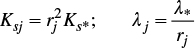(11)

where the subscript j identifies the soils: j=1,2,...,N, where N_s is the number of infiltration tests; r are the scale factors, and the parameters with asterisks correspond to the reference soil.

From equation, we infer:

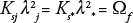(12)

where parameter Ω_f [L³T^-1] is a constant characteristic of the study region. Equation (12) allows reducing the number of unknown parameters of 2N_s to N_s+1 (^{Zataráin et al., 2003}). Because hydraulic conductivity at saturation is independent of the water depth over the soil surface and of the initial condition, the scaling provided by equation (12) should be written as:

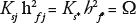(13)

where the new regional parameter Ω is estimated considering the definition of parameter λ, from:

Fuentes (1992)⁴ suggested that the reference soil be constructed in such a way that its hydraulic conductivity to saturation be equal to the geometric mean; that is:

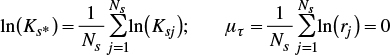(14)

where μ_τ is the arithmetic mean of the logarithms of the scale factors: τ =ln(r).

The fit of the scaled experimental data and the Green and Ampt function to the parameters of the reference soil show the applicability of the theory of similar media to the experimental information (Figure 2).

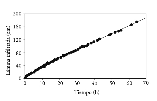
Figure 2 Scaled experimental data and Green and Ampt function with parameters of the reference soil (^{Zataráin et al., 2003}). 

Experimental data (^{Nielsen et al., 1973}; ^{Warrick and Amoozegard-Fard, 1979}; ^{Sharma et al., 1980}; ^{Vauclin, 1982}) show that it is valid to consider that the variable τ=ln(r) exhibits Gauss distribution. Considering the normalization defined by equation (14), the Gaussian probability density p(τ) and accumulated probability F(τ) are written as follows:

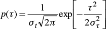(15)

(16)

where σ_τ is the standard deviation of the logarithm of the scale factors, and erf(x) denotes the error function.

In the scaling conducted by ^{Zataráin et al. (2003}), the following parameters of the reference soil were obtained: K_s*=2.33 cmh^-1 and λ_*=7.71, and regional: Ω=5.84 cm³h^-1. Spatial variability is reflected in the values of the scale factors, with mean ‹r›=1.0231 and standard deviation ‹σ_r›=0.2217. By assuming that, in effect, the variable τ=ln(r) follows a Gauss distribution, we determined that σ_τ=0.2207. Saturated hydraulic conductivity had a mean ‹K_s›=2.55 cmh^-1 and standard deviation ‹σ_Ks›=1.08 cmh^-1, which also illustrates the spatial variability of the hydrodynamic properties along the length of the border strip. The standard deviation of the saturated hydraulic conductivity in the border strip studied here is of the same order of magnitude as those found in the literature (Kutilek and NielTo analyze the spatial structure of the logarithm of the scale factors, the auto-correlogram and the semivariogram are introduced. The auto-correlogram, or function of autocorrelation of a process z(x), with second order stationarity and mean μ, is defined as:

(17)

where h is the distance between two points. The autocorrelation coefficient is defined as ρ(h)=C(h)/ σ² with the variance σ² =C(0), and is such that |ρ(h)|≤1. In the case of this study, z(x)= τ(x), σ²= σ_τ² and μ=μ_τ=0.

The semivariogram is defined as:

(18)

From equations (17) and (18) it is inferred that the semivariogram divided by the variance is related to the autocorrelation coefficient:

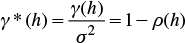(19)

To calculate the semivariogram or auto-correlogram, the following unbiased estimator was used:

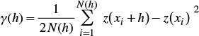(20)

where N(h) is the number of pairs of points separated by a distance h.

To model the empirical semivariogram, we applied the first order Markovian hypothesis, which results from the autocorrelation coefficient:

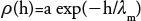(21)

where λ_m is the length of autocorrelation. For the data of the border strip studied, ^{Zataráin et al. (2003}) assumed that ρ(0)=a=1, which permits estimating a length of autocorrelation λ_m=10.

Effective properties

To establish the conditions in which the advance phase can be described by effective characteristics, ^{Zataráin et al. (2003}) considered that a) infiltration has a steady regime over long times; Darcy flow is equal to saturated hydraulic conductivity (K_s); b) the mean (K¯^s) exists; and c) spatial variability of the hydrodynamic characteristics in the advance phase is manifested fully over very long times, that is, when the flow regime approximates the steady regime.

A steady infiltration regime allows establishment of limt→∞ xf⁡(t)= xmax and limt→∞ Uf⁡(t)= 0, and U_f(t)=dx_f/dt [LT│^-1] is the advance rate. When t→∞, the Saint-Venant wave is completely established, the depth no longer depends on time ∂h/∂t=0 and _I, equation (1) is reduced to dq/dx+K_s(x)=0, whose integration leads to (q=0 in x=x_max):

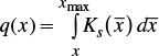(22)

and at the entrance of the border strip (x=0, q=q₀) we have:

(23)

According to the mean value theorem for integrals, the mean over the interval [0, x_max] is defined as:

(24)

That is:

(25)

Equation (25) indicates that, for a given irrigation flow rate, there is a mean value of hydraulic conductivity that defines a position of the maximum advance front. For a border strip of L length, the minimum flow rate that assures that the water will arrive at the end is deduced from equation:

(26)

Considering that the conductivity mean is a constant over the interval [0, L], K-s(L)= Ks, representation of the advance phase with effective hydrodynamic characteristics, that is, regardless of the intake flow, is possible for flows larger than that provided by equation (26).

Generation of correlated fields

Generation of a correlated field of hydraulic conductivity consists of producing realizations of the same that have certain imposed characteristics. For the case of the second order stationarity hypothesis, it is sufficient to maintain the mean and the semivariogram (^{Journel and Huijbregts, 1978}).

The methods grounded in spectral analysis permit generating a realization z(x) at any point in space (^{Rice, 1954}; ^{Shinozuka and Jan, 1972}; ^{Mejía and Rodríguez-Iturbe, 1974}). Spectral analysis of a random function z(x) associates the autocovariance function C(h) to its Fourier transform, called spectral density S(ω), where ω is the angular frequency, namely:

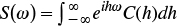(27)

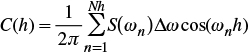
By analogy to the case of a random temporal phenomenon, in the case of spatial random functions, a spectral generator is used to simulate the function, that is:

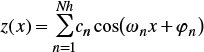(28)

where Nh is the number of harmonics; c_n is a coefficient of ponderation that permits the restitution of the spectral density function of the signal and its variance; ω_n are the signal frequencies; φ_n are the random phase angles distributed uniformly between 0 and 2π; cos(ω_nx + φ_n) is a random phase model, second order stationary, ergodic, of null mean and variance equal to a half.

The autocovariance function that results from the introduction of equation (28) into equation (17) is the following:

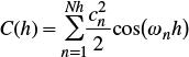(29)

where ω_n are the frequencies of each of the harmonics.

From equation (29), the following expression of the variance C(0)= σ² is obtained:

(30)

Among the methods proposed for estimating the coefficient c_n is that of ^{Mejía and Rodríguez-Iturbe (1974}), which assumes that all of the coefficients are equal and obtains cn = σ2Nh the variance is conserved, but not all of the semivariogram (Muñoz-Pardo, 1987)⁵.

In our study, the method of ^{Shinozuka and Jan (1972}) was chosen because it conserves the spatial structure and the variance. From the inverse Fourier transform of spectral density, equation (27) is deduced (^{Falconer, 1990}):

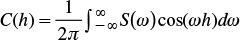(31)

which is discretized as follows:

(32)

and as C(0)= σ², we deduce that:

(33)

where Δω=2Ω/Nh in such a way that -Ω<ω_n<Ω.

Comparison of equations (30) and (33) leads to the following expression to calculate the coefficients:

(34)

Results and Discussion

The general conditions for representing soil hydrodynamic properties with effective parameters to simulate surface irrigation were analyzed by synthetic parameter generation. Initially, correlated hydraulic conductivity fields were generated using the logarithm of the scale factors and the ^{Shinozuka and Jan (1972}) method. The values were introduced into the hydrological model simulating the advance front. Then, the probabilistic parameters were used to generate parameters of random infiltration in the soils, considering that the general condition for using effective hydrodynamic properties in surface irrigation implies that the probabilistic distribution of the hydrodynamic properties are unique in space.

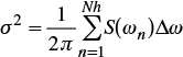
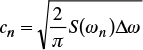
The realizations conserve the variance and the semivariogram. To illustrate, results were obtained with five generated correlated fields (Figure 3) and we observed that the probabilistic distribution of the logarithm of the scale factors was conserved. Behavior of the semivariograms of the generated fields was similar to the theoretical semivariogram within the scale of correlation (Figure 4).

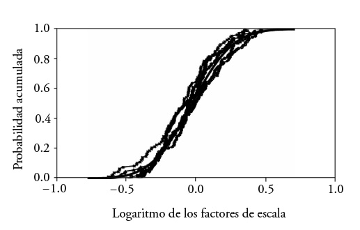
Figure 3 Accumulated probability of the logarithm of the scale factors in the Montecillo border strip and in generated correlated fields. 

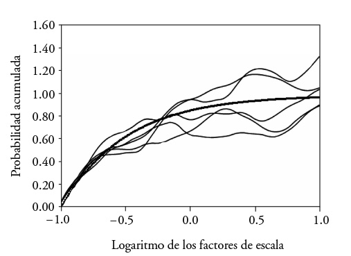
Figure 4 Theoretical semivariograms and of the correlated fields of the logarithm of the scale factors. 

The values of the scale factors of the five correlated fields (Figure 5) were introduced into the irrigation advance simulation model.

Figure 5 Spatial distribution of the five fields of generated scale factors. 

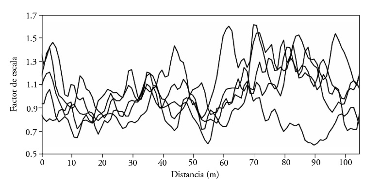
The scale factors of the correlated fields were introduced into the irrigation advance simulation model with the reference values K^*_s=2.33 cmh^-1 and λ ^*=7.71, with whichh^*_f=27 cm was obtained. The slope of the border strip was J₀=0.002 mm^-1, and saturated water content was υ_s=0.4865 cm³cm^-3; initial moisture was θ_o=0.2479 cm³cm^-3, and unitary flow was q₀=0.032 m³s^-1m^-1.

To select the parameters k and d of the law of hydraulic resistance, with equation (6) the Reynolds number was calculated Re=Uh/υ=q/υ to estimate the type of flow regime. With υ=10^-6 m²s^-1, Rc=3200 was obtained, allowing use of the Law of Poiseuille (d=1) of the depth regime (^{Sotelo-Ávila, 1997}). The average value of the depth at the head of the border strip was h_o=2.07 cm. With equations (8) and (9), were obtained k ≅ 1/54 y h- ≅ 1.38 cm

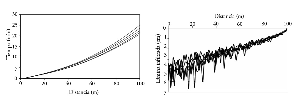
The advance front simulated with the five correlated fields was similar to experimental data (Figure 6).

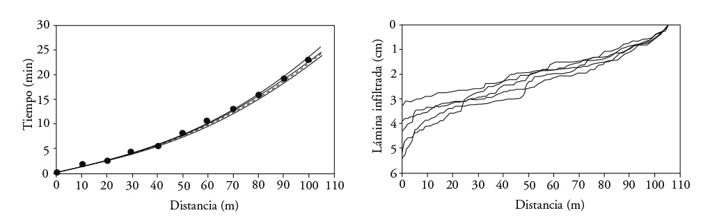
Figure 6 Advance and infiltration in the Montecillo crop bed with correlated fields of hydraulic conductivity using the logarithm of scale factors. 

Despite the spatial variability of the correlated fields, reflected in the profile of infiltrated depths, the simulation of irrigation advance showed practically the same behavior. Thus, the application of correlated fields permits contributing to analysis of conditions for applying inverse methods in the characterization of soils with irrigation events.

The probabilistic parameters were also used to study the general conditions that represent hydrodynamic properties by effective properties. This condition implies that the probabilistic distribution of hydrodynamic properties is unique in space. Modeling the advance is done by varying the number of soils from two up to one hundred. For each value of the number of soils, at least 10 replications are done of the advance modeling. In each replication, scale factors, whose number corresponds to the number of soils, are generated randomly; that is, each soil is represented by its scale factor.

To obtain the scale factors, probability values for the soils were generated randomly and, with the accumulated probability function, the logarithm values of the scale factors were obtained. The same reference soil as in previous cases was used. The values were placed, as they were being generated, over the 100 m border strip and discretized for modeling in 100 nodes. Intake flow rate was 3.2 ls^-1m^-1. The number of nodes per soil resulted from dividing the total number of nodes by the number of soils.

In a border strip with two soils with hydrodinamic contrasting characteristics, half the border strip was clay soil (r=1.434) and the other half was sandy soil (r=0.678). In the first case, the clay soil was placed at the beginning of the border strip, and for the second, sandy soil was placed at the beginning. Advance time was higher in the second case due to the greater volume that infiltrated (Figure 7).

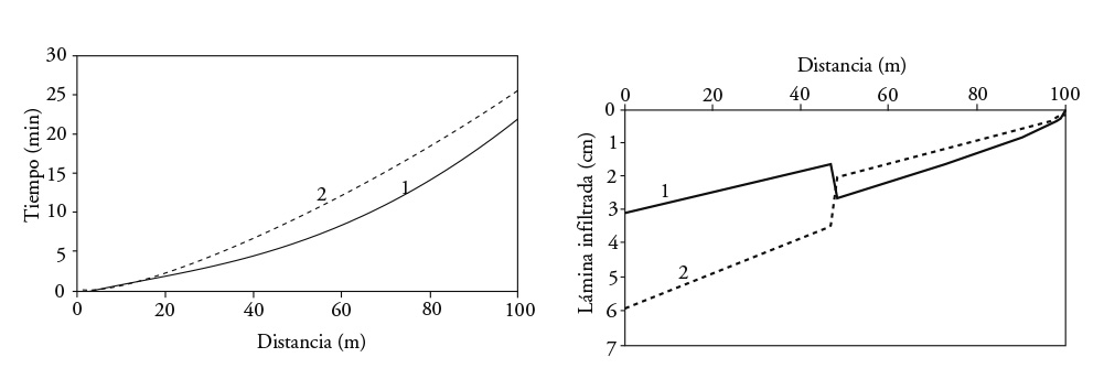
Figure 7 Advance curve and infiltrated depth in a border strip with two soil combinations: 1) clay-sand and 2) sand-clay. 

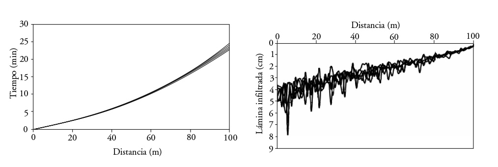
In modeling with 20, 50 and 100 soils, we observed that when the number of soils increased, the advance curves were more similar (Figures 8, 9 and 10). When the number of soils increased, total advance time oscillated, converging to a single value (Figure 11).

Figure 8 Advance curve and infiltrated depth in a border strip with twenty soil types. 

Figure 9 Advance curve and infiltrated depth in a border strip with fifty soils. 

Figure 10 Advance curve and infiltrated depth in a border strip with 100 soils. 

Figure 11 Total irrigation advance time obtained from modeling and synthetic generation of soils. 

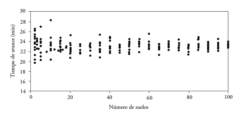
Modeling with two soils, interchanging their position, showed a large difference in advance times. With the increase in number of soils, advance time converged into a single value. This confirmed that, to model the advance phase in surface irrigation, effective hydrodynamic properties exist when their probability distribution is unique.

Conclusions

Analysis of the conditions in which the advance phase in surface irrigation can be modeled with effective hydrodynamic properties was approached by reproducing spatial variability of saturated hydraulic conductivity in two ways. One, with the creation of correlated fields that conserve the probability distribution and spatial structure through a method grounded in spectral analysis; and two, with random generation using the same probability distribution. With both procedures, it was possible to confirm that it is valid to use equivalent parameters of hydrodynamic properties of the soils when the probability distribution is unique in space. This conclusion is important since even in soils with spatial variability, equivalent parameters can be determined to permit prediction of flow and distribution of water in an irrigation event. For this purpose, inverse methods can be used with models based on the equations of Barré de Saint-Venant for surface flow and of Richards for subsurface flow, or with their simplified forms using hydrodynamic irrigation tests and considering the aspects inherent to inverse methods, which involve estimation of parameters, minimizing one objective function with an optimization algorithm over the deviations between observed and simulated flow variables

REFERENCES

Angulo-Jaramillo, R., J.-P. Vandervaere, S. Roulier, J.-L. Thony, J.-P. Gaudet, and M. Vauclin. 2000. Field measurement of soil surface hydraulic properties by disc and ring infiltrometers: A review and recent developments. Soil Till. Res. 55:1-29. [ Links ]
Bautista, E., and T. S. Strelkoff. 2009. Soil and crop hydraulic properties in surface irrigation. J. Irrig. Drain. Eng. 135:523-524. [ Links ]
Castanedo, V., H. Saucedo, y C. Fuentes. 2013. Comparación entre un modelo hidrodinámico completo y un modelo hidrológico en riego por melgas. Agrociencia 47: 209-223. [ Links ]
Durner, W., U. Jansen, and S.C. Iden. 2008. Effective hydraulic properties of layered soils at the lysimeter scale determined by inverse modelling. J. Soil Sci. 59: 114-124. [ Links ]
Falconer, K. 1990. Fractal Geometry, Mathematical Foundations and Applications. John Wiley & Sons. England. 288 p. [ Links ]
Fuentes, C., B. de León, H. Saucedo, J.-Y. Parlange, y A.C.D. Antonino. 2004. El sistema de ecuaciones de Saint-Venant y Richards del riego por gravedad: 1. La ley potencial de resistencia hidráulica. Ingeniería Hidráulica en México 19: 65-75. [ Links ]
Green, W. H., and G. A. Ampt. 1911. Studies in soil physic, 1: the flow of air and water through soils, J. Agric. Sci. 4: 1-24. [ Links ]
Journel, A. G. and Ch. J. Huijbregts. 1978. Mining Geostatistics. Academic Press, New York. 612 p. [ Links ]
Jury, W. A. et al. 2011. Kirkham’s legacy and contemporary challenges in soil physics research. Soil Sci. Soc. Am. J. 75:1589-1601. [ Links ]
Kutilek, M., and D. R. Nielsen. 1994. Soil Hydrology. CATENA VERLAG. Germany. 370 p. [ Links ]
Lewis, M. R., and W. E. Milne. 1938. Analysis of border irrigation, Trans. of ASAE 19: 267-272. [ Links ]
Mejía, G., and I. Rodríguez-Iturbe. 1974. On the synthesis of random fields from the spectrum: An application to the generation of hydrologic spatial processes. Water Resour. Res. 10: 705-711. [ Links ]
Mesgouez, A., S. Buis, S. Ruy and G. Lefeuve-Mesgouez. 2014. Uncertainty analysis and validation of the estimation of effective hydraulic properties at the Darcy scale. J. Hydrol. 512:303-314. [ Links ]
Miller, E. E., and R. D. Miller. 1956. Physical theory for capillary flow phenomena. J. Appl. Phys. 27: 324-332. [ Links ]
Nielsen, D. R., J. W. Biggar, and K. T. Erh. 1973. Spatial variability of field measured soil-water properties. Hilgardia 42: 215-259. [ Links ]
Parlange, J.-Y., R. D. Braddock, I. Lisle, and R.E. Smith. 1982. Three parameter infiltration equation. Soil Sci. 111: 170-174. [ Links ]
Parlange, J.-Y ., R. Haverkamp, and J. Touma. 1985. Infiltration under pounded conditions: 1. Optimal analytical solution and comparison with experimental observations. Soil Sci. 139: 305-311. [ Links ]
Rendón, L., C. Fuentes, y G. Magaña. 1997. Diseño del riego por gravedad. In: Robles Rubio, B. D. (ed.) Manual para el Diseño de Zonas de Riego Pequeñas. Instituto Mexicano de Tecnología del Agua, México. [ Links ]
Rice, S. O. 1954. Mathematical analyses of random noise. In: Wax, N. (ed.) Selected papers on noise and stochastic processes. Dover Publications: New York. [ Links ]
Richards, L. A. 1931. Capillary conduction of liquids through porous mediums. Physics 1: 318-333. [ Links ]
Saucedo, H., C. Fuentes, y M. Zavala. 2006. El sistema de ecuaciones de Saint-Venant y Richards del riego por gravedad: 3. verificación numérica de la hipótesis del tiempo de contacto en el riego por melgas. Ing. Hidrául. Méx. 21: 135-145. [ Links ]
Sharma, M. L., G. A. Gardner, and C. G. Hunt. 1980. Spatial variability of infiltration in watershed. J. Hydrol. 45: 101-122. [ Links ]
Shinozuka, M., and C. M. Jan. 1972. Digital simulation of random processes and its applications. J. Sound. Vib. 25: 111-128. [ Links ]
Sotelo-Ávila, G. 1997. Hidráulica general. ed. Limusa, México. 561 p. [ Links ]
Strelkoff, T.S., A.J. Clemmens, and E. Bautista. 2009. Estimation of soil and crop hydraulic properties. J. Irrig. Drain. Eng. 135: 537-555. [ Links ]
Vauclin, M. 1982. Méthodes d’étude de la variabilité spatiale des propriétés d’un sol. In: Institut national de la recherche agronomique, Société hydrotechnique de France and Groupe de travail "Dispersion en milieux poreux". Variabilité spatiale des processus de transfert dans les sols. Serie: Colloque S.H.F.-I.N.R.A. Paris: Institut national de la recherche agronomique. p. 9-43. [ Links ]
Warrick, A. W., and A. Amoozegard-Fard. 1979. Infiltration and drainage calibration using a similar media concept. Water Resour. Res. 13: 355-362. [ Links ]
Zhu, J., and B. Mohanty. 2006. Effective scaling factor for transient infiltration in heterogeneous soil. J. Hydrol. 319:96-108. [ Links ]
Zataráin, F., C. Fuentes, L. Rendón, y M. Vauclin. 2003. Propiedades hidrodinámicas efectivas del suelo en el riego por melgas. Ing. Hidráu. Méx. 18: 5-15 [ Links ]
4Fuentes, C. 1992. Approche fractale des transferts hydriques dans les sols non-saturés. Thése Docteur, L’Université Joseph Fourier de Grenoble. France. 267 p.
5Muñoz-Pardo, J. F. 1987. Approche géostatistique de la variabilité spatiale des milieux géophysiques. Application a l’echantillonnage de phénoménes bidimensionnels par simulation d’une fonction aléatoire. Thèse Docteur-Ingènieur, L’Université Scientifique, Technologique et Médicale de Grenoble. 254 p.
Received: December 2015; Accepted: July 2016
Este es un artículo publicado en acceso abierto bajo una licencia Creative Commons