


 texto en
  Inglés (pdf)
 Artículo en XML
 Referencias del artículo
 Enviar artículo por email
 Citado por SciELO
  Similares en
SciELO
Similares en
SciELO 
 Permalink
Introduction
A hydrological model may be defined as the mathematical representation of the water cycle on a portion of the Earth, in order to perform rainfall-runoff transformations. Hydrological models can be classified into lumped, and distributed (Carpenter and Georgakakos, 2006). A lumped model performs a simplified water balance, using single parameters that represent an average of spatial variability of the characteristics of a relatively large area. Distributed models divide the basin into smaller subareas, considering the spatial variability of the data and model parameters (Garcia et al., 2008). The concepts of lumped and distributed models, while opposite in meaning, are not necessarily exclusive, because a lumped model may be used as components of a distributed model (Ponce, 1989).
The time scale of simulation may be hourly, daily, weekly, or monthly. When the simulation is performed continuously in an hourly or daily time scale, the majority of the processes involved in the water cycle require a large number of parameters. By contrast, simulations based on weekly or monthly time intervals require fewer parameters (Garcia et al., 2008).
The implementation of a model requires an initial phase to collect the set of variables necessary for the mathematical representation of the physical phenomena. The number of parameters increases depending on the detail of the mathematical model used in the representation of the physical phenomena. When the number of parameters is large, it is necessary to perform a sensitivity analysis prior to calibration.
Through the systematic change of the values of the model parameters, and a detailed observation of the effects that these changes have on the results, a small number of calculation-relevant “sensitive” parameters are selected. In turn, these are tuned in during calibration until the model is able to reproduce the historical record in an acceptable manner.
After calibration, the model may be used to study different scenarios of climate change, land use, and so on. When a model is lumped and of monthly time scale, a low volume of information is required for implementation, which; has helped to increase the popularity of the lumped models in regions with limited information. The Temez model (Temez, 1977; Estrela, 1999) is used in Ibero-America for modeling rainfall-runoff in medium-sized watersheds with different climatic and geographical conditions (Murillo et al., 2005; Pizarro et al., 2005;Murillo and Navarro, 2011). Meanwhile, the SWAT model is applied successfully to flow and sediment simulation, in medium-scale and large-scale basins, in regions of Latin America, with varied weather and topographic conditions (Rivera-Toral, 2013; Oñate-Valdivieso and Bosque, 2014; Salas-Martinez, 2014).
The aim of this study was to evaluate the performance of the Temez hydrological model in the prediction of runoff in six sub-basins at the border between Ecuador and Peru and compare its performance with the performance of SWAT model.
Materials and Methods
Study area
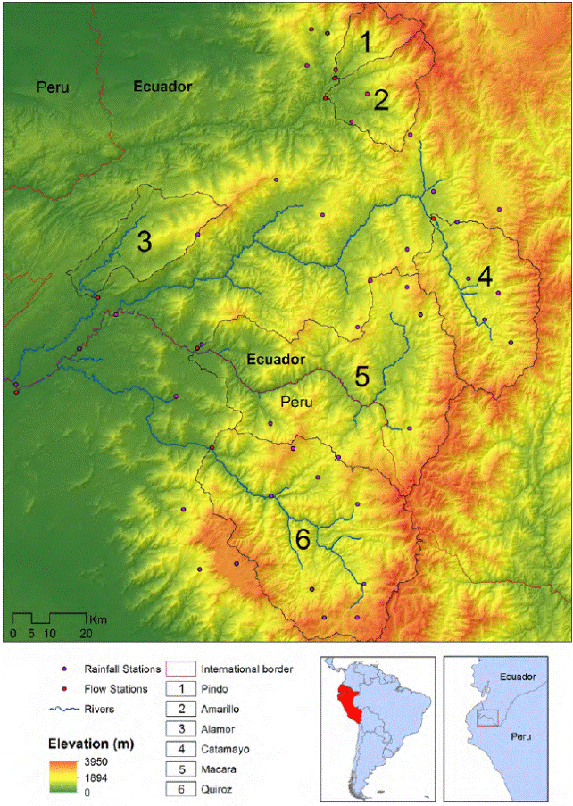
Six basins were selected, located between 3° 30’ and 5° 8’ S and 79° 10’ and 80° 29’ W, which belong to the bi-national basins Catamayo-Chira and Puyango-Tumbes, located along the border between Ecuador and Peru.
The Catamayo-Chira Binational Basin has an extension of 17 199.19 km2 and 817 968 inhabitants. The basin begins in the mountains of the Continental Divide (through Ecuador) and it ends in the Pacific Ocean (Peru). It goes through the Andes Mountain range downwards to the coast. It features tropical weather, diverse ecosystems, and various administrative/political systems. The geography of the basin is abrupt, with altitudinal variations between 0 m and 3700 masl and there are 11 life zones from tropical desert to mountain rainforest. The mean annual precipitation is about 800 mm, varying between 10 mm in the low-altitude areas to 1000 mm in the basin headwaters. Besides, 14 % of the basin surface is covered by humid forest, 41 % by dry forest, 30 % by pasture, 10 % by crops and 5 % by other uses.
The Puyango-Tumbes basin covers 5400 km2 and it includes the provinces of El Oro and Loja in Ecuador and the department of Tumbes in Peru. The upper basin consists of mountainous terrain with steep slopes, which elevations between 500 m and 3700 m, and encloses wilderness areas, natural forest and crops. The upper basin is characterized by an important mining activity, especially in Calera and Amarillo. The lower basin has extensive plains and it is heavily cultivated, with rice fields; there are also large areas of dry forests, grasslands, and agricultural crops. The lower basin in the Peruvian portion suffers from frequent floods. Precipitation in the basin ranges from 200 mm to 1150 mm per year, with average temperatures between 13 °C and 25 °C. Three main tributaries compose the basin: the Calera river, the Yellow River, and the Pindo river. On average, the total volume of water produced by the basin (average annual mass) is approximately 3,400 million m3.
The availability of hydrometric information and geographic characteristics determined the choice of six sub-basins: the basins from the Amarillo and Pindo rivers pertaining to the PuyangoTumbes basin, and the basins from the Catamayo, Macará, Quiroz and Alamor rivers pertaining to the Catamayo-Chira basin (Table 1). The geographic location of the basins is shown in Figure 1.
Table 1 Hydrographic basins chosen for model validation.
| Basin | Sub-basin | Gauging Station | Gaugin Station Coordinates | Basin area (km2) | Average flow (m3 s-1) | |
| Catamayo-Chira | Alamor | Alamor en Saucillo | 4° 15’ 31” S | 80° 11’ 42” W | 607.67 | 7.3 |
| Catamayo | Puente Boqueron | 4° 03’ 16” S | 80° 22’ 25” W | 1209.18 | 20.9 | |
| Macará | Puente International | 4° 23’ 00” S | 79° 56’ 60” W | 2641.69 | 37.1 | |
| Quiroz | Paraje Grande | 4° 37’ 48” S | 79° 54’ 48” W | 2275.76 | 15.3 | |
| Puyango-Tumbes | Amarillo | Amarillo en Portovelo | 3° 42’ 44” S | 79° 36’ 45” W | 262.31 | 14.32 |
| Pindo | Pindo Aj. Amarillo | 3° 45’ 40” S | 79° 38’ 01” W | 512.13 | 23.43 | |
Temez Model
The Temez Model (Temez, 1977; Estrela, 1999; Murillo and Navarro, 2011) is a lumped hydrologic model that assumes that the soil profile is divided into an unsaturated upper zone and a saturated lower zone. The model behavior is similar to that of an underground reservoir that drains into the surface network.
Rainfall (P) is divided into evapotranspiration (ET) and excess (T). The excess is decomposed into a fraction that flows over the surface (E) (surface runoff), and into another fraction that infiltrates into the ground (I). The first fraction evacuates through the channel within the established period of time, whereas the second will remain in the underground reservoirs to be released at a later time. The excess is calculated through the following expression:
in wich:
P t is the precipitation in the period between the instant i-1 to the instant i (mm); P 0 is the runoff threshold that defines the height of precipitation, under which no runoff is produced (mm); T t is the excess in the period between the instant i-1 to the instant i (mm); H max is the maximum capacity of soil moisture (mm); H i-1 is the soil moisture at the instant i-1 (mm); EP is the potential evapotranspiration from the instant i-1 (mm); and C is a parameter from the model.
The soil moisture, Hi, at the end of the period will result:
An actual evapotranspiration ER t (mm) is produced and it is equal to:
Equation 6 shows that all the water available can be evapotranspired, with the potential evapotranspiration as an upper limit.
The model adopts an infiltration amount (I t ) as a function of the excess, T t and of the maximum infiltration parameter, I max .
will be in mm.
The infiltration increases with the excess, being asymptotic for its higher values, having as a limit the I max value.
This infiltration, I i becomes recharge to the aquifer, R i , whereas the rest of the excess (E i = T i I i ) will become surface water. The model assumes that the time step in the unsaturated zone is lower than the simulation time step.
The draining of the aquifer is modeled by an exponential function of the following type:
where Q i is the discharge at the instant, i, α is the coefficient of the discharge branch of the aquifer that depends on the particular conditions of the basin being studied and t the time interval between instants i-1 and i.
The relation between the discharge Q i and the volume V i , stored in the aquifer is equal to:
The discharge for the infiltration is assumed to be concentrated in half of the time step; therefore, the law of the groundwater flow is:
in which R i is the discharge to the aquifer in the period between i-1 and i, coinciding with infiltration, I i .
The groundwater contribution throughout the period, A SUBi .
The total contribution, A Ti , is given by surface runoff (T i I i ) and the groundwater contribution:
There are four parameters of the model: Hmax, which is the maximum capacity of the soil moisture; Imax, maximum capacity of infiltration; C is the parameter of excess; a is the coefficient of the discharge of the aquifer. These four parameters are particular to each basin and are subject to calibration.
Soil and water assessment tool (SWAT)
SWAT is a continuous simulation model used to predict the impact of land management practices in the production of water, sediments, and nutrients in a watershed (DiLuzio et al., 2002). Besides, it is a semi-distributed continuous model based on the equation of water balance in the land profile and it simulates the precipitation, infiltration, runoff, evapotranspiration, lateral flow, and percolation processes. The equation of water balance is:
where SW t is the final soil water content (mm H2O), SW 0 is the initial soil water content on day i (mm H2O), t is the time (days), Rday is the amount of precipitation on day i (mm H2O), Q surf is the amount of surface runoff on day i (mm H2O), E a is the amount of evapotranspiration on day i (mm H2O), w seep is the amount of water entering the vadose zone from the soil profile on day i (mm H2O), and Q gw is the amount of return flow on day i (mm H2O).
The SWAT model accomplishes a topographic division of the basin into sub-basins based on threshold of area; in turn, the sub-basins are subdivided into one or more homogeneous hydrological response units (HRU) that represent a unique combination of soil type and land use. The response to each HRU in water, sediments, nutrients, and pesticides are individually determined; then, they are added to a sub-basin level and moved toward the basin exit through its river network (Bouraoui et al., 2005).
The surface runoff is estimated from daily precipitation data using the curve number methodology or Green-Ampt equation (Neitsch et al., 2002). The evapotranspiration is determined applying the methodologies proposed by Hargreaves, PriestleyTaylor and Penman-Monteith (Neitsch et al., 2002). A kinematic reservoir that considers variations in hydraulic conductivity, prevailing slope, and soil moisture is used to predict the lateral flow in each one of its layers. Groundwater is divided in two aquifer systems: 1) a non-confined aquifer, which is shallow and contributes to the backflow; 2) a confined aquifer, which is deep and disconnected from the system, unless groundwater pumping is being considered (Bouraoui, et al., 2005). The sedimentation rate is estimated by applying the modified universal equation of soil loss (Neitsch et al., 2002), using for that purpose the surface runoff, peak flow rate, erodibility of soil, slope length, its inclination, crop factor, and the management practice in the zone. Neitsch et al. (2002) explained the theoretical basis of the SWAT model.
Implementation, calibration, and validation of the model
For each basin, the lumped modeling was performed considering as input data the average spatial rainfall in the basin and the monthly potential evapotranspiration. For calibration purposes, the monthly average flows recorded in the downstream station of each basin included in Table 1 were considered. The precipitation data in 24 stations in Ecuador and in 19 in Peru stations as well as the temperature data in 10 stations in Ecuador and 4 stations in Peru were considered. The correspondence of the data series was verified through double-mass curve analysis. By regression analysis between stations that present geographical closeness, the same climatic regime, and the compatibility of records, data were homogenized to the common period 1970-2000 in the stations of the Catamayo-Chira basin, and 1965-1995 in the station of the Puyango-Tumbes basin. The Thornthwaite method (Thornthwaite and Mather, 1957) was used to calculate potential evapotranspiration in each one of the 14 stations for which the temperature data was recorded.
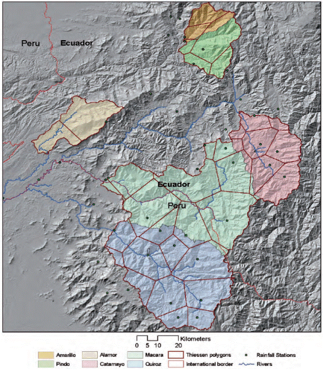
The average precipitation and evapotranspiration for each one of the basins were calculated by Thiessen polygons (Figure 2).
In each one of the selected basins, manual calibration of four parameters (C, Hma, Imax, a) of the Temez model was carried out based on successive approximations. For this calibration, 70% of the measured records were used; the flows calculated by the model were compared to the recorded flows in the stations included in Table 1. In the calibration process, the parameters values were changed to no more than 12%. Once the model parameters were calibrated, they were validated, generating flows for a period covering the remaining 30% of the historical record. The goodness of fit between the calculated and observed values was measured by calculating the correlation coefficient (R), the Nash-Sutcliffe model efficiency coefficient (EF) (Nash and Sutcliffe, 1970) and the root-mean-square error (RMSE). The correlation coefficient will measure the fit of the observed and calculated data to a straight line, the EF efficiency will measure the 1 to 1 relation of the observed data, and the RMSE will allow the evaluation of the average difference between observed and calculated values.
The application of the Temez model was performed by using the CHAC software which was developed by CEDEX of Spain. The Temez model may be found in http://hercules.cedex.es/ Chac/.
For comparison purposes, the SWAT model was implemented in each one of the sub-basins. A DEM from the Shuttle Radar Topography Mission (SRTM) of the study area was used for the delimitation of contributing basins and the calculation of the different morphometric parameters required by the model. Also, the information regarding the type of soil was gathered, and the soil parameters were determined by laboratory tests. Land use was extracted from a LANDSAT7 ETM+ image of October 2, 2011 through a supervised classification; in this extraction the minimum spectral angle (Chuvieco, 2002; Richards and Jia, 2006) was applied. The land use parameters were taken from the SWAT model database, with minor modifications. An existing soil type map (Valarezo, 2007) was validated and adapted for SWAT model implementation. The validation was done through perforations and pits in each of the edaphologic units identified. The infiltration test was performed in situ. Unaltered soil samples and general characteristics of soil horizons were taken. With all the collected data and the laboratory tests, the soil type parameters were determined for each of the edaphologic units identified.
The combination of soil type and land use allowed the determination of hydrological response units (HRU). The soil type information was used to characterize the non-confined aquifer. Additionally, precipitation and daily temperature data, as well as temperature parameters, solar radiation, wind speed, monthly relative humidity for each one of the stations were assembled to calculate evapotranspiration using the Penman Monteith method. The precipitation missing data were estimated by orthogonal correlation analysis between geographically neighboring stations with similar climatic conditions. In the case of temperature, an elevation-temperature equation was determined. A similar process was used for other climatic variables.
Before calibration, an analysis of model sensitivity was made by systematically changing the values of the model parameters and watching for the effect that such changes have on the obtained results, by selecting a reduced number of sensitive parameters of a higher relevance in the calculation and optimizing them in the calibration phase. The sensitive analysis was made using the module that the SWAT model has for this purpose, which combines the Latin hypercube sampling method with the one factor at a time (OAT) simulation (van Griensven et al. 2006). The Latin hypercube sampling method, in opposition to the conventional Monte Carlo method, makes a stratified sampling between the rank of possible values of each parameter; moreover, the OAT simulation assures that changes in the model can be attributed to an change made to the entrance variable in each simulation (van Griensven et al. 2006).
The SWAT model was calibrated manually, adjusting the values of the most sensitive parameters changing its initial values to no more than 12%, using 70% of the gathered records, and optimizing R, EF, and RMSE. The SWAT model parameters about soil loss were not considered in the calibration process, because the Temez model does not reproduce sediment losses, so the comparison between Temez model and SWAT model was made only with flow data. The validation was performed with the 30 % remaining from the record. Finally, a graphic comparison of calculated and observed flows was carried out. See Oñate-Valdivieso and Bosque (2014) for additional information on the implementation of the SWAT model for basins study.
Results and Discussion
Calibration of parameters for the Temez model
The calibrated parameters for the Temez model in each one of the basins are shown in Table 2.
Table 2 Parameters for the Temez model calibrated for the studied basins.
| Sub basins | Excedance C | Maximum Humidity (Hmax) | Maximum Infiltration (Imax) | Branch of discharge α |
| Alamor | 0.1 | 400 | 400 | 0.01 |
| Amarillo | 0.3 | 80 | 200 | 0.03 |
| Catamayo | 0.3 | 200 | 400 | 0.01 |
| Macará | 0.1 | 200 | 380 | 0.08 |
| Pindo | 2.0 | 150 | 230 | 0.02 |
| Quiroz | 0.8 | 150 | 200 | 0.01 |
The maximum capacity of soil moisture (Hmax) allows the definition of the threshold runoff (Po), i.e., the rainfall below which there is no runoff; thus, the excess (Ti) is defined and it is composed of the runoff and infiltration into the aquifers. Table 2 shows that the values of Hmax surpass 150 mm in most of the cases, reaching a maximum value of 400 mm. The values of this parameter show a high storage capacity of the soils in the surveyed zone, which experience a considerable water deficit during most of the year. This situation can be found at the sub-basin of the Alamor river. The opposite can be observed at the subbasin of the Amarillo river, which is dry in its lower section but shows higher levels of rainfall throughout the year. For this reason, soils are more humid and have a lower maximum capacity of infiltration.
The parameter of excess C is used to determine the runoff threshold P o and acts as a weighting factor of the difference between the maximum humidity of the soil and its humidity at a given moment. The values of parameter C (Table) 2 are lower than 1; thus, controlling a possible sub-estimation of the excess produced when considering relatively high humidity factors.
The actual infiltration I is directly proportional to the maximum infiltration I max , the former being a fraction of the latter. Additionally, the values of this parameter, which are included in Table 2, show a level of maximum infiltration corresponding with H max . Since this is an arid zone, high levels of infiltration may be expected.
The coefficient α reaches average values between 0.01 and 0.08. This parameter is related to the contributions of groundwater flow to the base flow of the basins analyzed. The higher values can be found in the basins with a larger area, since these basins extend across zones with different levels of contribution of groundwater. In higher zones, which are usually more humid and exhibit better conditions of plant growth, the contribution of groundwater is higher, unlike lower zones, where the opposite occurs. The calibrated parameter in the larger basins is representative of such conditions.
Evaluation of the Temez model
The parameters used to determine the goodness of fit between the observed and calculated flows for the period of validations are included in Table 3. The graphical relation between observed and calculated flows using the Temez model is shown in Figure 3.
Table 3 Analysis of goodness of fit of Temez model. Summary of the calculated parameters.
| Sub-basin | Area (km2) | R | EF | RMSE |
| Amarillo | 262.00 | 0.64 | 0.63 | 7.32 |
| Pindo | 512.00 | 0.63 | 0.49 | 14.47 |
| Alamor | 607.67 | 0.72 | 0.35 | 9.11 |
| Catamayo | 1209.00 | 0.48 | -0.82 | 10.72 |
| Quiroz | 2275.76 | 0.69 | 0.62 | 23.94 |
| Macará | 2641.69 | 0.82 | 0.27 | 53.01 |
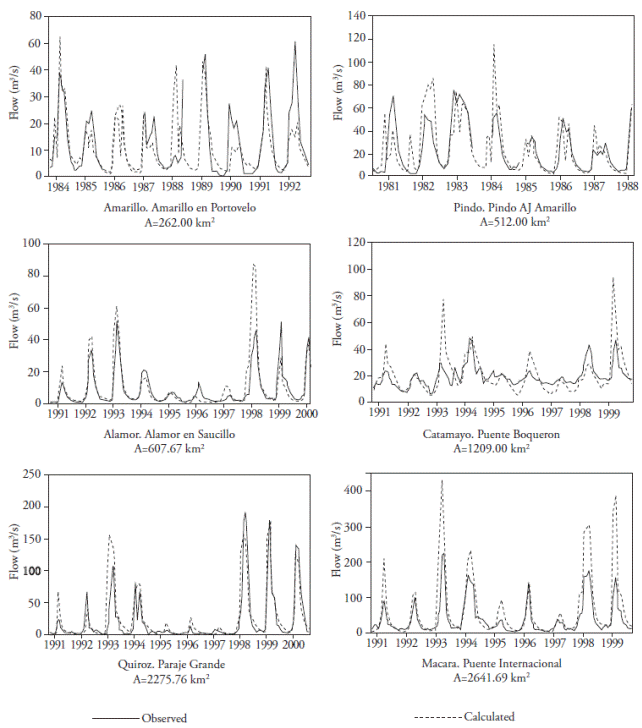
In smaller basins (Amarillo, Pindo and Alamor), the model recreates the flows of the dry season better than those of the rainy season (Figure 3). As the size of the basin increases, an overestimation of the flows may be observed, and the correspondence between observed and calculated flows almost disappears. The overestimation of flows is due to the calculation of the flow as the product of the contribution (mm per month) multiplied by the area of the basin assuming that the levels of rainfall and evapotranspiration are uniform across the basin. This does not necessarily apply to medium-sized or large basins.
The Amarillo river basin shows a correlation coefficient of 0.64 and an efficiency EF of 0.63 (Table 3). These values confirm the existence of an acceptable adjustment between the observed and calculated values. The average quadratic error is 7.32 m3 s-1, which, if compared to the average flow recorded (14.32 m3 s-1), is excessive. In Figure 3, it is shown that the model does not accurately recreate peak flows, and the flows of the dry season are overestimated.
In the Pindo river basin, which approximately doubles the size of the Amarillo river basin, there was a correlation coefficient of 0.63 between the observed and calculated data, which is barely acceptable; besides, EF was 0.49, which is lower than that observed in the Amarillo river basin. The average quadratic error is 14.47 m3 s-1, which, if compared to the average flow of the Pindo river (23.43 m3 s-1), turns out to be excessive. The model overestimates flows. As shown in Figure 3, the best adjustment is produced in the flows of the dry season, and the peak flows shows the worst adjustment.
In the Alamor river basin (Table 3) there was a relatively good correlation between calculated and observed values (R=0.72); however, there is a low value of EF (0.35), with an average quadratic error of 9.11 m3 s-1 that surpasses the average observed flow of 7.3 m3 s-1. It could be expected that with a high correlation coefficient RMSE should be lower, but as shown in Figure 3, the model recreates the trend; therefore, the value of the correlation coefficient is satisfactory. In addition, the recorded peak flows are overestimated to a great extent by the model and this has an influence on RMSE. The EF exhibits a more realistic value of 0.35, which, although it is not optimal (EF=1), it gives an idea of the model’s performance, which is, to a certain extent, acceptable.
The Catamayo river basin station (Table 3) presents the worst results, which means that there is no correlation between observed and calculated flows. A negative value of the Nash-Sutcliffe efficiency is obtained; it can be considered that the mean of the observed values is a better predictor than the model itself.
The Quiroz river basin shows acceptable values of the correlation coefficient (R=0.69) and the NashSutcliffe efficiency (EF=0.62), although the excessive average quadratic error, which duplicates the average observed flow, shows the overestimation of the calculated flows.
The Macara river basin has the best correlation coefficient (R=0.82); however, the low value of the Nash-Sutcliffe efficiency (EF=0.27) implies that the model cannot recreate the hydrological behavior of the basin. In addition, the average quadratic error almost doubles the average observed flow by overestimating flows in general.
The study area is mainly mountainous, with irregular rainfall and since the average number of rainfall station is only one every 270 km2, and it is assumed that the existing network of meteorological stations in the area does not have sufficient density to accurately reflect the spatial variability of precipitation. Additionally, historical records of precipitation, temperature and especially flow, showed significant information gaps that, to some extent, point to problems in the management of meteorological and hydrological stations in the area.
Like precipitation, slope, soil type, and land use present a significant spatial variation. Therefore, considering a single lumped value, representative of each condition may be strictly valid only for very uniform and small basins.
Comparison with SWAT model
Meteorological data was the most difficult to achieve in the study area, because the number of weather stations is low, only 14. Information about wind speed, solar radiation and relative humidity was the scarcest.
The sensitivity analysis reported the 35 most sensitive parameters, which were classified in a scale of 35 levels and 1 corresponds to the most sensitive parameter. Table 4 shows the first 10 parameters reported by sensitivity analysis and their influence levels in the model.
Table 4 Sensitive parameters of SWAT model.
| Parameter | Symbol | Ranking |
| Moisture condition II curve number | CN2 | 1 |
| Biological mixing efficiency | BIOMIX | 2 |
| Average slope | SLOPE | 3 |
| Surface runoff lag coefficient | SURLAG | 4 |
| USLE support practice factor | USLE_P | 5 |
| Available water capacity | SOL_AWC | 6 |
| Linear parameter for calculating the maximum amount of sediment that can be reentrained during channel sediment routing | SPCON | 7 |
| Moist soil albedo | SOL_ALB | 8 |
| Soil evaporation compensation coefficient | ESCO | 9 |
| Baseflow recession constant | ALPHA_BF | 10 |
As shown in Table 4, the model turned out to be sensitive to the curve number CN2 because this parameter is used to separate effective precipitation from total precipitation. Therefore, there is a direct effect on the runoff calculation; furthermore, the available water capacity SOL_AWC determines surface runoff since it causes higher or lower infiltration. The Baseflow recession constant ALPHA_ BF will regulate the contributions of groundwater to the flow. The moist soil albedo SOL_ALB and the soil evaporation compensation coefficient ESCO regulated losses by evapotranspiration. An important influence was observed in the average slope SLOPE and the surface runoff lag coefficient SURLAG, thus directly affecting the concentration time of each subbasin and varying the temporal occurrence of peak flows. The soil loss parameters were not considered
A graphical analysis of the relationship between the observed flow and calculated flow with the SWAT model is presented in Figure 4. As seen in that figure, the SWAT model provides a better representation of trends and better fit with the observed values, even when considering the peak flows of the wet season and the low flows in the dry season.
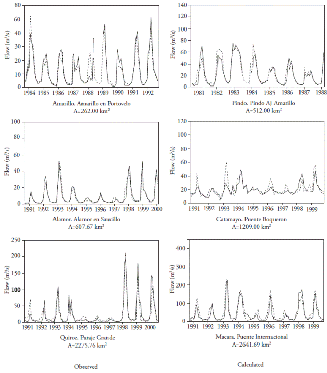
Comparative analysis of SWAT/ Temez model performance by validation parameters is summarized in Table 5. There it is observed that in all cases the SWAT model presents better correlation coefficient, reaching in most cases values higher that 80 %. The Nash-Sutcliffe efficiency is significantly higher when calculated with the values obtained with the SWAT model. Similarly, the RMSE was significantly smaller on values calculated with the SWAT model.
Table 5 Comparative analysis of SWAT/ Temez model performance by validation parameters.
| Sub basin | Gauging Station | Model | R² | EF | RMSE |
| Pindo | Pindo Aj. | TEMEZ | 0.63 | 0.49 | 14.47 |
| Amarillo | SWAT | 0.86 | 0.80 | 9.07 | |
| Amarillo | Amarillo en | TEMEZ | 0.64 | 0.63 | 7.32 |
| Portovelo | SWAT | 0.88 | 0.87 | 4.29 | |
| Alamor | Alamor en | TEMEZ | 0.72 | 0.35 | 9.11 |
| Saucillo | SWAT | 0.85 | 0.84 | 4.43 | |
| Quiroz | Paraje Grande | TEMEZ | 0.69 | 0.62 | 23.94 |
| SWAT | 0.83 | 0.83 | 16.19 | ||
| Catamayo | Pte. Boqueron | TEMEZ | 0.48 | -0.82 | 10.72 |
| SWAT | 0.55 | 0.20 | 7.07 | ||
| Macará | Pte. Internacional | TEMEZ | 0.82 | -0.27 | 53.01 |
| SWAT | 0.81 | 0.77 | 22.64 |
As a semi-distributed SWAT model, a better performance in all of basins may be expected. However, even though in the smaller basins, the Temez model performance is lower to that of the SWAT model, which could be acceptable considering the lower amount of information required for implementation of the Temez model.
Considering that in many places the lack of information is a reality, the Temez model may be a viable option when applied to a relatively small watershed. Additionally, the Temez model could be used as a basis for a semi-distributed model applicable to larger watersheds.
Conclusions
The Temez model showed some effectiveness in reproducing the flow in dry seasons, with very low effectiveness in reproducing the flows in the rainy season. The correlation coefficient, the efficiency of Nash-Sutcliffe and RMSE were less than satisfactory in most of the basins studied.
The overall accuracy of the results decreased with an increase in watershed area. The moderate effectiveness shown by the Temez model can be attributed to the low density of the network of weather stations, which are unable to properly characterize precipitation and temperature. A lumped model with monthly intervals over simplifies the natural process and it does not reproduce correctly the behavior of the basin.
The SWAT model showed better simulation capabilities, due to the nature of its semi-distributed simulation, but its implementation required a large amount of information, which in some cases may not be readily available.
The Temez model showed simulation capabilities lower to those of SWAT model with a large number of parameters. The Temez model may be efficient in areas with low spatial variability of input data and model parameters, so its use in small basins may be indicated.
Acknowledgements
The authors would like to express their gratitude to the Secretaría Nacional de Ciencia, Tecnología e Inovacion of Ecuador (SENESCYT) for funding this research through its scholarships program.

