Introduction

Trade liberalization and economic integration of Mexico have grown since they joined the General Agreement on Tariffs and Trade (GATT) in 1986 and the North American Free Trade Agreement (NAFTA) in 1993. In 2013 the country had a network of 10 Free Trade Treaties with 45 countries, 30 agreements for the Promotion and Reciprocal Protection of Investments and nine Agreements of Limited Scope (Economic Complementation Agreements and Partial Scope Agreements) under the Latin American Integration Association (ALADI). Mexico in 2013 had a degree of commercial openness of 64 %. So when the GDP size is considered it ranks as one of the world's most open economies, only exceeded by relatively small countries.

Although in the recent 10 years, purchases from the US have declined at an average annual growth rate (AAGR) of 2 %, and imports from China and Europe have increased at an AAGR of 10 % and 0.3 % each; in 2013 Mexico's trade relations were mainly with the US, totaling 52 % of its imports and 82 % of its exports.

In the trade flow analysis exports are closely related to economic growth, although the flow is not highly correlated with the recovery of the economic cycles of the industrial and semi-industrial countries, exports are under the assumption of the export - led recoveries hypothesis (^{Feder, 1983}; ^{Prasad and Gable, 1998}; ^{Irwin and Terviö 2002}; ^{Tekin, 2012}). Because the agricultural sector is made up of highly traded products and the large trade liberalization that Mexico has experienced in recent 15 years, the RER has become an important variable for the analysis of sector development.

The RER is a relative price and as such is not under direct control of the authorities, but there are several macroeconomic and sectoral policies that affect it (^{Sadoulet and De Janvry, 1995}); therefore, it can be influenced through policy measures. ^{Eichengreen (2008)} stated that these should be focus on promoting a stable environment and the alignment of macroeconomic policy with sectoral objectives.

Studies on the determination of the exchange rate recognize its importance in the economy. The article by ^{Schuh (1974)} allowed considering the role of the exchange rate as a fundamental variable to explain commercial flux, especially the agricultural. They stressed that the exchange rate plays a key role in the development of international trade, primarily agricultural, in the resources assessment and the distribution of the benefits of economic progress between consumers and producers within an economy.

The exchange rate is the most powerful influence on the relative prices of the economy and its effects on real agricultural prices exceed those of other types of price intervention (setting maximum and minimum prices), it is also one of the main instruments used for macroeconomic stabilization (^{Sadoulet and De Janvry, 1995}).One reason why agriculture is most susceptible to the exchange rate variability is that its products are highly traded or that are close substitutes regarding production or consumption of export or import products (^{Norton, 2004}).

Despite the decline in the relative importance of agricultural exports, these are relevant in regional terms, in the labor market and the restart of the domestic demand. The agroindustry has the best performance, showing positive growth rates even during times of crisis, which shows the high potential of this sector.

There are several studies on the exchange rate in Mexico, these are focused on predictability and management (^{Loría, 2003}; ^{Bahmani-Oskooee and Hegerty, 2009}; ^{Loría et al., 2010}; ^{Ramírez and Arreola, 2013}). However, a structural model of the exchange rate indicating the fundamental variables that determine their behavior has not been developed.

Among the most mentioned variables in studies with econometric models with predictive application of the exchange are: capital flows (^{Rozo, 1997}), interest rate (^{Clarida and Waldman, 2007}; ^{Engel et al., 2007}; ^{Chaboud et al., 2008}; ^{Chen and Tsang, 2010}) and monetary aggregates (^{Don and Lee, 1987}; ^{Loría et al., 2010}; ^{Bahmani, 2011}).

The studies on the exchange rate determination have used real and nominal variables, highlighting the PD as an explanatory value (^{Miyakoshi, 2003}; ^{Choudhri and Khan, 2005}; ^{Guo, 2010}); the differential in the interest rates, associated to the volatility of the exchange rate (^{Miyakoshi, 2003}; ^{Bagchi et al., 2004}; ^{Chen, 2006}); TI cointegrated with the RER (Bagchi et al., 2004; ^{Aizenman and Riera-Crichton, 2008}; ^{Bleaney and Francisco, 2010}); the O, arguing that an increase of this variable will lead to significant depreciation of currencies of net oil-importing countries in relation to the currencies of net oil-exporting countries (^{Chen and Chen, 2007}; ^{Korhonen and Juurikkala, 2009}; ^{Lizardo and Mollick, 2010}); international reserves, which show a significant effect in developing economies, where they ease the TT impact on the RER, observing a direct relationship between these variables (^{Wang and Dunne, 2003}; ^{Aizenman and Riera-Crichton, 2008}); and capital flows which show a significant effect, especially in developing economies (^{Aizenman and Riera-Crichton, 2008}).

In the search of the variables that determine the exchange rate through the study of the longitudinal behavior of time series, different methodologies are used: 1) Markov focus shift (^{Chen, 2006}), 2) analysis systems by autoregressive models (^{Goldberg and Frydman, 1996}; ^{Faust et al., 2007}; ^{Fang et al., 2009}), 3) spectral analysis (^{Grossmann and Orlov, 2012}), and 4) co-integration (^{Kim, 2003}). The results depend on the characteristics of each studied country, the degree of liberalization and trade dependence, specialization, relative importance of each productive sector and government policies.

^{Ramírez and Arreola (2013)} indicated that the time series of the Mexican exchange rate cannot be analyzed with generalized autoregressive conditional heteroskedasticity models (GARCH) due to the irreversibility of this variable in time. These kinds of models are valid with univariate structures and in the study of the impact of a treatment. However, from a theoretical perspective it is more appropriate, especially for multivariate models, the dynamic modeling system including cointegration analysis (^{Rosel et al., 1999}).

Cointegration techniques in the study of the exchange rate were used by ^{Baillie and Selover (1987)}, ^{Kim and Mo (1995)}, ^{Kim (2003)} and ^{Bagchi et al. (2004)}, highlighting its use in forecasting. In our study, a multivariate model that used series that, in theory and empirically are important in determining the RER between Mexico and the US, was utilized and using the cointegration techniques, specifically the methodology of ^{Engle-Granger (1987)}, for the the econometric model.

This study was conducted under the assumption that the RER is influenced by TT, the RD, PD and O. The objective was to determine through the econometric analysis the impact of key variables that affect the behavior of the RER between Mexico and the US to provide the basis for successful government intervention.

Materials and Methods

Given the structural characteristics of the Mexican economy, the following variables were chosen: TT because they show the situation under which trade flows develops; RD because Mexico's exchange rate regime is not completely flexible; PD because it indicates the efficiency of resources usage; and O for its importance in the economy of Mexico.

For this study, annual data from 1980 to 2010 was used, period during which the exchange rate policy of Mexico had great dynamism. This period include the final stage of the industrialization Imports Substitution Model (ISI) and the beginning of trade liberalization in the 1990s.

The construction of the database used official information: Banco de Mexico (Banxico), National Institute of Statistics and Geography (INEGI), Ministry of Economy (SE) World Bank (WB), Bureau of Economic Analysis and Bureau of Labor Statistics (BLS). The series used were: the nominal exchange rate (pesos per dollar) obtained from historical daily exchange rate series peso-dollar from Banxico; the national consumer price index (CPI) 2005 for Mexico and the US built with information from the online consultation from INEGI and specific data series BM, respectively; price indices of exports and imports with based on 2005; GDP for Mexico and the US at 2005 prices and not seasonally adjusted; the amount of total reserves of Mexico and the US, all obtained from the BM; the economically active population (EAP) for US was that from the BLS database and the data for Mexico were the historical statistics published by the INEGI; and oil prices (Mexican crude and WTI) obtained by an electronic request at the website of the Mexican Geological Service of the Ministry of Economy.

Results and Discussion

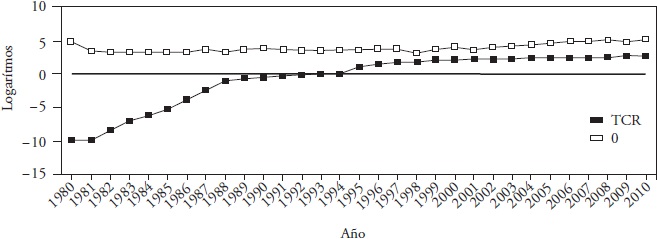
According to the graphical inspection of the 1980-2010 period data (Figure 1 and Figure 2) a cutoff period was distinguished in 1994 from which the RER series, the PD, RD and TT showed smaller variations; however, still maintain a tendency over time, indicating that they possess a unitary root. O appears to be a stationary series. The TT is the only variable that shows a downward trend.

Tests on stationarity reveal that the Q⁶ statistics are significant (α=0.001) and the absolute value of the ADF statistics that are lower than any of the critical values of ^{Mackinnon (1996)}, which forces to reject the null hypothesis that the RER, PD, RD, TT, O series are stationary. Therefore, the series possess unitary root in levels (Table 1).

Based on the non-stationarity of the data, it is not possible to estimate the parameters of the proposed model with the original series, because the estimated results could show spurious relationships. Therefore, the order of integration of each variable (Table 1), which indicates the number of times a time series has to be to distinguish to become a stationary series. In this way, a time series is integrated of order d, written I (d), if after differentiate it d times becomes stationary (^{Gujarati and Porter, 2010}).

The process of differentiation for each series is expressed as follows:

The results of these tests, both the original series and their first differences are in (Table 1), where evidence is shown to affirm that all series are non-stationary of order one I (1).

According ^{Gujarati and Porter (2010)}, two or more time series that are non-stationary of order I (1) are cointegrated if a linear combination exist that is stationary or of order I (0). The vector of coefficients that create this stationary series is the cointegrating vector. Since all series were integrations of order I (1), it is possible to inspect on the paired cointegration between RER and TT, PD, RD and O; the long-term equilibrium relations were established. The following long term RER static functions were specified and estimated:

The long-term relationship between each pair of variables was examined using the unitary root test ADF on the error term u_2,t as follows:

The null hypothesis H₀: non-stationarity of the disturbance (H₀: ρ=0), is tested against the alternative hypothesis H₁: stationary (H_a:ρ<0) through the t statistic for ρ.

The graphical inspection suggests that residues are stationary, i.e., with an order of integration I (0), except for the long term relationship between the RER and RD (Figure 3, 4, 5 and 6), which was corroborated by the statistics of the ADF test (Table 2). Therefore, the analyzed series tend to a long-term equilibrium with RER except for the PD series.

According to this, it is possible to estimate the parameters proposed by the OLS when the existence of a long-term relationship between the variables included in the model is verified.

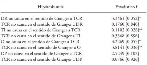
The Granger causality test was performed in order to confirm the direction of the relationship between the variables. Based on the probability values (Table 3), we cannot reject the null hypothesis that RER does not cause TT and that RER does not cause RD in a Granger direction. Never the less, the hypothesis that maintain that TT does not cause RER, that RD does not cause RER, that O does not cause RER and that RER does not cause O in the Granger sense is rejected. It follows the rejection of the null hypothesis that the RER variable precedes the variables O, TT and RD while O precedes RER. That is, the lagged values of the TT and RD variables have a significant impact on the endogenous variable RER, and between RER and O variables a feedback exists, ie the Granger causality runs in one direction, from TT to RER and from RD to RER and run in bidirectionally between RER and O.

According with the analysis on the behavior of the independent variables and their relation to the RER, the signs obtained in the parameters match the expected, except for O (Table 4).

The variables that are important to determine the RER are the RD, PD and O. The Granger causality test showed unidirectional causality from TT towards the RER; however, when estimating together with the other variables through OLS, the TT variable was not statistically significant.

The main results of the regression are:

For every percentage point the ratio of the reserves between Mexico and the US change, the RER change 0.85 % in a direct relation.

For each percentage point the real oil price change, the RER changes in 0.38 % in a direct relation.

In a net oil-exporting economy like Mexico, the increase in O leads to an appreciation (reduction) of the NER. The positive relationship found between O and RER is mainly explained by the relationship between the both US and Mexico inflation that deflated the NER. Higher oil prices improve the Terms of Trade of net export economy, so that the effect of the inflation from the importing country coupled with the actions of the Central Bank to prevent full NER mobility cause the direct relationship between O and RER.

For each percentage point the Terms of Trade change, the RER changes 0.57 % in an inverse relation.

Given that the dependent variable is in logarithmic scale and dummy takes the value 0 for the 19801993 period and 1 for the 1994-2010, its coefficient is used to calculate the percentage variation of the RER between the two periods (e^0.5243 - 1) 100) = 68.93 %. Since the dummy variable is statistically significant and since the 1994-2010 period coincides with a flexible rate regime (with the intervention of the Central Bank), the interpretation of this result is that such exchange rate regime in Mexico modified the RER level compared to the previous period in 68.93 %.

Although the RER is inelastic to changes in RD and O variables, it is through them that control and management of the RER can be exercised seeking its stability and alignment with the policy objectives.

Because the reserves management is a task of the monetary policy, the results of this study are consistent with others indicating that monetary policy has important effects on the behavior of the exchange rate, and it is an important mechanism for its management and control (^{Isik et al., 2005}; ^{Burstein et al., 2005}; ^{Kim, 2003}).

Conclusions

Although the terms of trade are co-integrated with the Real Exchange Rate, these do not serve as a fundamental explanatory variable of the behavior for the 1980 to 2010 period. However, the cointegration of the variables would allow them to be used in any other model. The productivity gap is an important variable in determining the Real Exchange Rate for developing economies; however, in the case of Mexico-U.S.A. It was not significant.

The Real Exchange Rate was inelastic to changes in the key variables, i.e., the percentage change in it is less than one for every percentage change in the Differential Reserves and the Oil Price. However, there is a direct relationship between the regressor and the regressand. A control strategy for the Real Exchange Rate should include monetary policy actions focused on the management of the international reserves.

Due to the bidirectional relationship between the real exchange rate and oil prices, and since this was statistically significant to determine the real exchange rate, it is useful to explore a simultaneous equations model that incorporates monetary policy variables like the interest rate in determining the oil prices.

The co-integration method for the analysis of the determinants of the RER allowed to specifying a model with independent variables that presented an equilibrium relationship in a long term with the RER. Such models are of interest to economic theorists who seek balance. With the ^{Engle-Granger methodology (1987)} the analytical approach of the econometric model is strengthened.