


Servicios Personalizados
Revista
Articulo
 texto en
  Inglés (pdf)
 Artículo en XML
 Referencias del artículo
 Enviar artículo por email
Indicadores
-
 Citado por SciELO
 -
 Accesos
Links relacionados
-
 Similares en
SciELO
Similares en
SciELO
Compartir

 Permalink
Agrociencia
versión On-line ISSN 2521-9766versión impresa ISSN 1405-3195
Agrociencia vol.50 no.1 Texcoco ene./feb. 2016
Water-Soils-Climate
Meteorological variables prediction through ARIMA models
1Hidrociencias. Campus Montecillo. Colegio de Postgraduados. 56230. Montecillo, Estado de México. México. (aguado.graciano@colpos.mx), (anolasco@colpos.mx), (mcastro@colpos.mx).
2Irrigación. Universidad Autónoma Chapingo. 56230. Chapingo, Estado de México. México. (arteagar@correo.chapingo.mx), (mvazquezp@correo.chapingo.mx).
3Instituto Nacional de Investigaciones Forestales, Agrícolas y Pecuarias. Km. 13.5. Carretera Los Reyes-Texcoco. 56250. Texcoco, Estado de México. México. (zamora.patricia@inifap.gob.mx).
Meteorological variables prediction is applied in agriculture to predict water uptake of plants for planning irrigation depths. In the present study a program was made for the prediction of temperature, solar radiation, reference evapotranspiration and relative humidity by means of autoregressive integrated mobile media models. The effectiveness of the program was tested for prediction under high and low rainfall conditions. The prediction periods evaluated were in March and in June, 2013, in three automatic meteorological stations (EMAS) of the National Meteorological Service (SMN). The analysis of results indicated that the prediction of meteorological variables with ARIMA models was better than with persistent prediction in the period with low rainfall conditions (March).
Key words: Prediction; R Statistics; real time
La predicción de las variables meteorológicas se aplica en la agricultura al predecir el consumo de agua de las plantas para planear la lámina de riego. En esta investigación se elaboró un programa para realizar la predicción de la temperatura, radiación solar, evapotranspiración de referencia y humedad relativa con modelos autorregresivos integrados de media móvil (ARIMA) y se probó la efectividad del programa para realizar la predicción en condiciones de alta y baja precipitación. Los periodos de predicción evaluados fueron en marzo y en junio de 2013 en tres estaciones meteorológicas automáticas (EMAS) del Servicio Meteorológico Nacional (SMN). El análisis de los resultados indicó que la predicción de las variables meteorológicas con modelos ARIMA fue mejor que con la predicción persistente en el periodo con condiciones de baja precipitación (marzo).
Palabras clave: Prónostico; R Statictics; tiempo real
Introduction
There is great progress in the development and applications of medium term weather prediction and seasonal climate (Vitart et al., 2012). The most frequently used automatic prediction algorithms are based on the softened exponential or autoregressive integrated mobile media models (ARIMA) (Hyndman and Khandakar, 2008). Box and Jenkins (1976) developed the classic methodology that uses the time series for generating models such as the autoregressive mobile media model (ARMA) or also the ARIMA model for obtaining predictions.
Karl et al. (2000) found an increment in the global warming rate using the time series of global meantemperature indicated by Quayle et al. (1999), using the analysis of monthly values of temperature and with ARMA models. Reikard (2009) investigated the prediction of solar radiation in 5 min time intervals for various hours, and although the data exhibited non-linear variability due to cloudiness, in most of the tests best results were obtained using the RIMA models. Pulido (2002) proposed the estimation of water demand in the next 24 h in a water distribution system for irrigation using ARIMA and other models. To predict rainfall of the summer monsoon in India, Chattopadhyay and Chattopadhyay (2010) identified an ARIMA model as adequate, but the autoregressive neuronal network model (ARNN) provided better predictions, while Narayanan et al. (2013) used ARIMA models to predict rainfall prior to the monsoon in western India.
Because the ARIMA models are a tool used for univariate weather prediction, the present investigation was made with the purpose of elaborating a computer program that calculates prediction in real time of meteorological variables using ARIMA models and testing its effectiveness under low and high rainfall conditions.
Materials and Methods
The present investigation used a computer with a processor of 2.2 GHz, 2 GB of RAM memory and Windows 7® operative system. The following programs were installed: MySQL Server®, which is an administrator of data bases for storing information (Korhonen et al., 2008); Microsoft Visual Studio 2010®, which is a complete set of development tools for the generation of applications of Web ASP.NET, XML Web Services, desktop and mobile applications (Randolph et al., 2010); MySQL Connector Net 6.3.5® which is a connector of the program Microsoft Visual Studio 2010® with MySQL Server (Kofler, 2005); R Statistics 2.15.3®, computer statistical package (Dalgaard, 2008); ‘rcom’ and ‘rscproxy’ libraries of the program R Statistics 2.15.3 (connectors of the program R Statistics 2.15.3 with Microsoft Visual Studio 2010); and the ‘forecast’ library of the program R Statistics 2.15.3, which was used for the estimation and prediction of the ARIMA models.
To store meteorological information, a data base was made integrated with two data tables, in the program MySQL Server (Figure 1). The first data table was called ‘station’ and was used to store the information of each meteorological station, and for each station an identifier is required of station, latitude, longitude, altitude and name, and the primary key is the station identifier. The second data table, called ‘elemhoraria’ was used to store the information of the meteorological data at the time level of meteorological stations; the data stored in this table are: date and time, evapotranspiration (ET0 in mm), wind velocity (VELS in m/s), rainfall (mm), solar radiation (SOLRAD in W/ m2), mean temperature (TEMP in °C), relative humidity (RH in %), and an identifier of the station from which the data is from: the primary key is joining the data of date and station identifier.
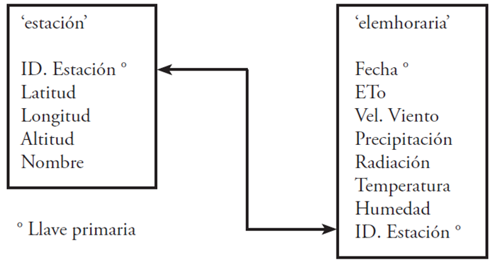
In Figure 1, it is observed that a station can have many records at the hourly level and many stations can have meteorological data for a particular hour.
Meteorological data
To test the predictive goodness of the ARIMA models, data were used from three automatic meteorological stations (EMAS) of the National Meteorological Service, Mexico, for 2013. The EMAS considered were as follows: ENCB. II of the IPN, located at 19° 29’ 55” N, 99° 08’ 43” W and altitude of 2240 m; Acolman, located at 19° 38’ 05” N, 98° 54’ 42 W and altitude of 2269 m; Chapingo, located at 19° 29’ 39” N, 98° 53’ 19” W and altitude of 2260 m.
In the EMAS for this study there are continuous data at the hourly level of five meteorological variables in two periods: the first is of March 7, 2013 at 16:00 h and March 17, 2013 at 15:00 h; the second is of June 16 , 2013 at 16:00 h and June 26, 2013 at 15:00 h. The meteorological variables obtained from the EMAS were as follows: wind velocity (m/s), rainfall (mm), solar radiation (W/m2), mean temperature (°C), relative humidity (%). In addition, reference evapotranspiration (ET0) was calculated by the Penman Monteith method (Allen, 2006) with the above data.
ARIMA Models
According to Pankratz (1983), the ARIMA models serve to predict simple series (of a single variable), in which the predictions of the ARIMA models are based only on past values of the variable for prediction. The ARIMA models can be used to make short term predictions because most of them place more emphasis on the recent past than on the distant past; they are applied to discrete or continuous variables, although time should be equally spaced and in discrete intervals; they are useful for predicting data series that contain seasonal variation (or other periodic variations), including those with changing seasonal patterns; they require a minimum of 50 observations; it is applied only to series of stationary data, and a series of stationary time has a mean, variance and function of autocorrelation that are constant through time (Pankratz,1983).
The requirement of a stationary time series may seem totally restrictive, but most of the non-stationary series in practice can be transformed into a stationary series through a process called “differentiation”, which is a relatively simple operation that involves the calculation of successive changes in the values of the data series. The changes in the data series are known as (wt) and are obtained with the equation wt=zt-zt-1, where z represents the values of the data series. With the differences a new series is constructed, different from the original, and a “difference” is when the mean of a series of data changes with time. It is possible to “differentiate” more than just once to obtain a stationary series. When a stationary series is obtained, a good ARIMA model is sought and consists of : identification, estimation, diagnostic of the model, and if the model is adequate the prediction is made (Pankratz, 1983).
Description of the procedure of the Forecast library for estimating the ARIMA model
According to Hyndman et al. (2013), a common obstacle when using ARIMA models for prediction is that the selection process of the order is generally considered subjective and difficult to apply. Therefore, the Forecast library was made to select the order of the model automatically, and where the algorithms are applicable to both stationary and non-stationary data.
For Hyndman et al. (2013), a non-stationary ARIMA process (p,d,q) is obtained by:
where {εt} is a white noise process with mean zero and variance s2, B is the delay operator, and Ø(z) and Ø(z) are polynomials of order p and q, respectively. To insure causality and invertibility, it is assumed that Ø(z) and Ø(z) do not have roots for |z|<1. If c≠0, there is an implicit polynomial of d order in the prediction function. The seasonal process ARIMA(p,d,q)(P,D,Q)m is obtained as follows:
where Ø(z) and Ø(z) are polynomials of order P and Q, respectively, neither one containing roots within the unitary circle. If c≠0, there is an implicit polynomial of order d+D in the prediction function.
The principal task of the Forecast library that Hyndman et al. (2013) carry out in the automatic prediction of the ARIMA model is to select an appropriate order of model and they are the known values of p, q, P, Q, d. If D and d are known. The orders p, q, P, and Q can be selected by means of a criterion of information such as the Akaike Information Criterion (AIC):
where k=1 if c≠0 and 0 otherwise, and L is the maximized probability of the model fitted to the differentiated data (1-Bm)D (1-B)dyt.
For purposes of prediction, Hyndman et al. (2013) point out that it is better to make the fewest differences possible. For non-seasonal data, Hyndman et al. (2013) consider ARIMA (p,d,q) models where d is selected based on the test of successive unitary roots KPSS (Kwiatkowski et al., 1992). The method tests the data for a unitary root; if the result of the test is significant, differentiated data are tested for a unitary root; and so on.
For seasonal data, in the Forecast library ARIMA(p,d,q) (P,D,Q)m models are considered where m is the seasonal frequency and D = 0 or D = 1, depending on an extended test of Canova-Hansen(Canova and Hansen, 1995). After selecting D, d is selected applying the test of successive unitary roots KPSS to the differentiated seasonal data (if D =1) or to the original data (if D=0).
Estimation of the prediction
With Microsoft Visual Studio 2010 a usable application was developed (.exe), with which functions are made for the prediction of the meteorological variables. However, before describing these functions it is important to emphasize that most of the EMAS have the option of downloading the information they record and saving it in text files. Therefore, a first function was made for extracting the data of the meteorological variables stored in text files (of each EMAS) and storing them in the data base. The meteorological data are stored in the data base at the schedule level of different EMAS and are organized by date and identifier of EMA; the data obtained are stored in the data table ‘elemhoraria’. Its function is also used to calculate reference evapotranspiration by the Penman Monteith method (Allen, 2006) and the result is stored in the same data table.
When the first function is completed, the averages of the meteorological variables are obtained at the hour level in the data base. The second function is used to generate a time series for each meteorological variable of the three EMAS, and the resulting time series contains 60 data. Each data of the time series consists of the average of two hours. For example, if for day 16/06/2013 at 16:00, 17:00, 18:00 and 19:00 the average temperature was 22, 23.7, 24.7 and 24.8 °C, respectively, and on June 21 of 2013 at 14:00 and 15:00 h the average temperature was 16.2 and 15.6 °C, respectively, then the time series will have the values 22.85, 24.75, …, 15. °C, with a total of 60 data. The generated time series are stored in a text file created automatically with extension ‘.txt’ for each EMA (Figure 2). The file has six columns (one column for each meteorological variable) and 61 days. The first row contains the names of the meteorological variables; however, only four variables are analyzed. The first variable is in the first column and has the data of reference evapotranspiration (mm), the fourth column has the data of solar radiation (W/m2), the fifth column contains the data of temperature (1C) and the sixth column includes the data of relative humidity (%).
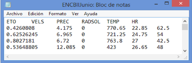
Figure 2 Content of the text file with time series of meteorological variables for the EMA ENCBII for the period of June.
When the second function is finished, we have obtained the time series for each meteorological variable necessary for carrying out the prediction. The prediction is obtained with the third function. In the first step of the third function a connection is established between the program R Statistics 2.15.3 and Microsoft Visual Studio 2010; the programming language was C#. Then a command is sent to the program R Statistics 2.15.3 to fit the time series of each meteorological variable to an ARIMA model using the function “auto.arima” of the Forecast library (Hyndman et al., 2013). Next, using the automatically estimated ARIMA model, a command is sent to the program R Statistics 2.15 to make the prediction of the next 60 elements in the time series.
The function “auto.arima” of the Forecast library (Hyndman et al., 2013) gives back the best ARIMA model. However, the function “auto.arima” requires arguments such as a univariate time series, the order of the first difference “d” (if it is not put in, the function “auto.arima” selects a value according to the KPSS test), the order of the first seasonal difference “D” (if it is not put in, the function “auto.arima” calculates it), the maximum value for p, q, P, Q, the initial value of p, q, P, Q (optional), if the time series is stationary, if the time series is seasonal, among other optional data.
For the function “auto.arima” the options were specified of maximum value of p equal to 5, maximum value of q equal to 5, and the seasonal option equal to “TRUE”, because otherwise the search for non-seasonal models is restricted. The last function consists of saving the predictions obtained with the function “auto.arima”. To carry this out, text files are created with extension ‘.txt’ where the predictions are stored. The name of the file is created with the combination of the name of the EMA, the name of the variable and the word PRED at the end (to indicate that it is prediction). Figure 3 shows the name of the file generated of the station ENCBII for the variable air temperature.
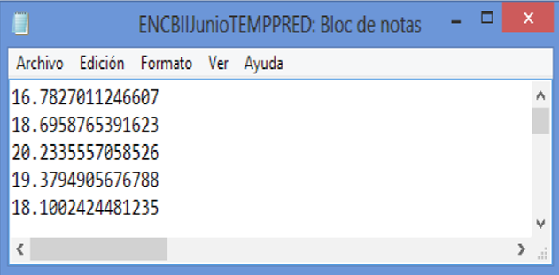
Figure 3 File generated with data of the prediction estimated with the function "auto.rima" for the EMA ENCBH in the period of June of the meteorological variable air temperatura (°C)
In the text file generated by the prediction (Figure 3), in the first line, the prediction of the average of the variable between 16:00 and 17:00 h on June 21 of 2013, in the second line is the prediction of the average of the variable between 18:00 and 19:00 h on June 21 of 2013, and in the last row of the file is the prediction of the average of the variable between 14:00 and 15:00 h of June 26 of 2013.
Results and Discussion
The precision of the prediction in the two periods was evaluated. In the first, the data observed between March 7 of 2013 at 16:00 h until March 12 of 2013 at 15:00 h were used to generate the time series, and the data observed between March 12 of 2013 at 16:00 and March 17 of 2013 at 15:00 h were used to be compared with the data estimated with the prediction model. Next, the precision of the prediction in the second period was evaluated. The data observed between June 16 of 2013 at 16:00 h and June 21 of 2013 at 15:00 were used to generate the time series. The data observed between June 21 of 2013 at 16:00 h and June 26 of 2013 at 15:00 h were used to compare with the data of the estimated predictions.
In Figures 4 and 5 the observed data were graphed with the estimated data of the meteorological variables: relative humidity (%), air temperature (°C), solar radiation (W/m2) and reference evapotranspiration (mm) . The data obtained as observed from reference evapotranspiration were calculated with the method of Penman Monteith (Allen, 2006) and using the observed data of the other meteorological variables.
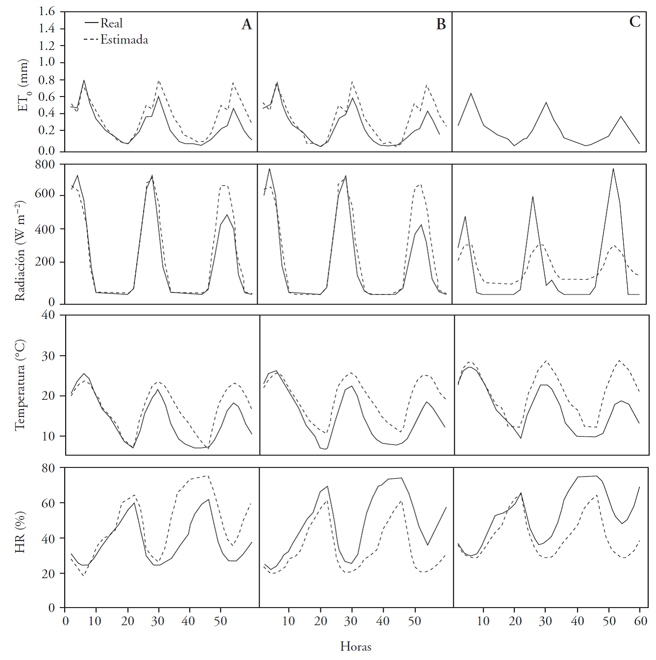
Figure 4 Prediction and variables observed 60 h ahead for the EMA Acolman (A), Chapingo (B), and ENCB. II of the IPN (C) in the first period (March).
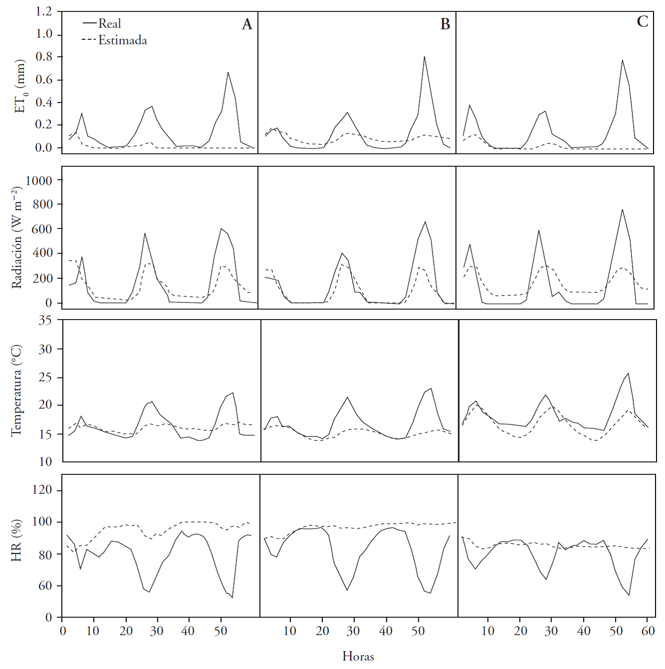
Figure 5 Prediction and variables observed 60 h forward for the EMA Acolman (A), Chapingo (B), and ENCB II of the IPN (C) in the second period (June).
The ARIMA models obtained for each station and meteorological variable are found in Table 1
Table 1 ARIMA models for the time series of the meteorological variables evapotranspiration (ET0), relative humidity (RH), solar radiation (SOLRAD) and air temperature (TEMP).
| Estación | Variable | Ø 1 | Ø 2 | θ 1 | θ 2 | θ 3 | Φ 1 | Θ 1 | ARIMA(p,d,q)(P,D,Q) 12 |
|---|---|---|---|---|---|---|---|---|---|
| Acolman | ET0 | 0.38 | -0.58 | ( 1, 0, 0 )( 1, 1, 0 ) | |||||
| Chapingo | ET0 | 0.68 | ( 1, 0, 0 )( 0, 1, 0 ) | ||||||
| ENCBII | ET0 | Sin ajuste | |||||||
| Acolman | HR | 0.86 | 0.69 | 0.45 | -0.67 | ( 0, 0, 3 )( 1, 1, 0 ) | |||
| Chapingo | HR | 1.11 | -0.35 | -0.28 | ( 2, 0, 0 )( 1, 1, 0 ) | ||||
| ENCBII | HR | -0.44 | -0.45 | ( 0, 1, 1 )( 0, 1, 1 ) | |||||
| Acolman | RADSOL | 0.81 | -0.26 | -0.72 | ( 2, 0, 0 )( 1, 1, 0 ) | ||||
| Chapingo | RADSOL | 0.40 | -0.25 | -0.67 | ( 2, 0, 0 )( 1, 1, 0 ) | ||||
| ENCBII | RADSOL | -0.27 | ( 0, 0, 1 )( 0, 1, 0 ) | ||||||
| Acolman | TEMP | -0.61 | ( 0, 1, 0 )( 0, 1, 1 ) | ||||||
| Chapingo | TEMP | 1.45 | -0.62 | -0.43 | 0.97 | -0.50 | ( 2, 0, 1 )( 1, 0, 1 ) | ||
| ENCBII | TEMP | 0.76 | ( 0, 0, 1 )( 0, 1, 0 ) | ||||||
| Periodo de junio | |||||||||
| Acolman | ET0 | 1.63 | -0.87 | -1.68 | 0.78 | 0.73 | ( 2, 1, 2 )( 1, 0, 0 ) | ||
| Chapingo | ET0 | 1.19 | -0.51 | -0.96 | 0.57 | ( 2, 1, 1 )( 1, 0, 0 ) | |||
| ENCBII | ET0 | 0.22 | 0.60 | ( 0, 1, 1 )( 1, 0, 0 ) | |||||
| Acolman | HR | 0.34 | 0.68 | ( 1, 1, 0 )( 1, 0, 0 ) | |||||
| Chapingo | HR | 0.35 | 0.38 | ( 1, 1, 0 )( 1, 0, 0 ) | |||||
| ENCBII | HR | 0.72 | -0.50 | -0.42 | 0.36 | ( 1, 1, 2 )( 1, 0, 0 ) | |||
| Acolman | RADSOL | 1.23 | -0.55 | 0.83 | ( 2, 0, 0 )( 1, 0, 0 ) | ||||
| Chapingo | RADSOL | 0.62 | 0.52 | 0.89 | -0.39 | ( 1, 0, 1 )( 1, 0, 1 ) | |||
| ENCBII | RADSOL | 1.02 | 0.50 | 0.80 | -0.37 | ( 0, 0, 2 )( 1, 0, 1 ) | |||
| Acolman | TEMP | 1.38 | -0.63 | 0.64 | ( 2, 0, 0 )( 1, 0, 0 ) | ||||
| Chapingo | TEMP | 1.66 | -0.91 | -1.67 | 0.72 | 0.29 | ( 2, 1, 2 )( 1, 0, 0 ) | ||
| ENCBII | TEMP | 0.41 | 0.04 | -0.35 | -0.56 | 0.95 | -0.75 | ( 1, 1, 3 )( 1, 0, 1 ) | |
For a given time series {y n }, the persistent prediction is obtained by placing y(n+1)=y(n), which implies that the average of the variable for the next hour is equal to the average of the variable in the present hour (Kavasseri et al., 2009).
To compare the predictive goodness of the ARIMA models with the persistent prediction, measurements of the error and of the mean square of the error (MSE) were calculated. Cadenas and Rivera (2007) point out that is the value observed in the time t is y t and Ft is the prediction for the same time, then the error is defined as e t =y t - F t , and the mean square of the error is:
In our study the observed value of the average of air temperature between 16:00 and 17:00 of March 12, 2013, was 20.7 °C and the value obtained with the prediction of the ARIMA model for the same time was 19.96 °C, thus the MSE of the ARIMA model of that time was 0.547. The value of the persistent prediction of this same time was 14.95 (the observed value of the average of the air temperature between 14:00 and 15:00 h of March 12, 2013); therefore, the value of the MSE of the persistent model of this time was 33.06. The same operation was carried out for the 40 h ahead (20 times ahead).
The MSE value MSE was calculated from 5 in 5 times ahead for all of the variables (5, 10, 15, 20, etc) until the value of the MSE obtained with the prediction of the ARIMA models (MSEA) was higher than the value of the MSE obtained with the prediction of the persistence model (MSEB). In the air temperature variable of the period of March of the Acolman station, it was found that up to 15 times ahead the value of MSE A (2.531) was lower than that of the MSEB (10.309); and at 20 times the value of MSA (11.204) was higher than that of MSB (10.422). To compare the errors, a percentage of improvement of prediction was calculated of the ARIMA model with respect to the prediction with the persistent model.
The percentage of improvement of the prediction of the ARIMA model with respect to the prediction with the persistent model (PM) was calculated as follows:
where MSEA is the MSE of the ARIMA model, MSEP is the MSE of the persistent model.
In the variable of air temperature of the period of March at the Acolman station and 15 times ahead, it was found that the value of PM was 75.4 %, which indicates that the ARIMA model performs 75.4 % better than the persistent model as far as 15 times ahead (30 h). Thus, the calculation of the PM was made for all of the meteorological variables in both periods (March and June) and for the three EMAS (Table 2).
Table 2 Percentage of improvement of the prediction of the ARIMA model with respect to the precision with the persistent model (PM) for meteorological stations Acolman (A), Chapingo (B), and ENCBII (C), the times ahead (T) and in the periods of March and June.
| PM(%) | |||||||||
|---|---|---|---|---|---|---|---|---|---|
| Marzo | Junio | Promedio | |||||||
| Variable | T | A | B | C | A | B | C | Marzo | Junio |
| ET0 | 20 | 51.4 | 55.7 | ---- | -153.3 | -42.6 | -56.1 | 53.6 | -84.0 |
| HR | 15 | 65.7 | 27.7 | 49.5 | -408.8 | -425.3 | -135.3 | 46.7 | -323.1 |
| RADSOL | 30 | 83.3 | 64.9 | 65.0 | 19.1 | 13.1 | 23.8 | 71.0 | 18.7 |
| TEMP | 15 | 75.4 | 33.0 | 21.7 | -42.0 | -140.8 | 4.9 | 43.4 | -59.3 |
Two important aspects in a prediction plan are:
1) how well a model retains its precision over the prediction horizon, and 2) how robust is the plan for the selection of the prediction horizon (Kavasseri et al., 2009). To observe the first aspect, predictions were made of the values of the meteorological variables ahead until the PM was less than zero. When the values of PM are less than zero, it indicates that the MSEP was better than the MSEA (the prediction with the persistent model was better than with the ARIMA model). To observe the second aspect, two periods were selected: the period of March with very little precipitation (less than three rainfall events and less than 1 mm total) and the period of June in which more than 20 rainfall events occurred (more than 8 mm total).
The ARIMA model predicts better than the persistent model more than 15 times ahead for the variables ET0, RH, SOLRAD and TEMP in the period of March (Table 2). For the period of June it was found that the persistent model was better than the ARIMA model for the variables ET0, RH and TEMP. A possible reason for this is that rainfall affects the other meteorological variables and can change the behavior of a time series.
Conclusions
The use of computer software and ARIMA models allows the investigator to estimate the prediction of meteorological variables automatically and in real time. However, the results indicate that on the average, in the period of March with very little rainfall (less than 1 mm), prediction with the ARIMA models was better than prediction with the persistent model with: 53.6 % in reference evapotranspiration by as much as 20 times ahead (40 h); 46.7 % in relative humidity up to 15 times ahead (30 h); 71 % in solar radiation up to 30 times ahead (60 h); 43.4 % in air temperature as much as 15 times ahead (30 h). In the period of June, the predictions obtained with the persistent model were better than with the ARIMA model.
Literatura Citada
Allen, R. G. 2006. Evapotranspiración del cultivo: guías para la determinación de los requerimientos de agua de los cultivos. FAO 56: 89-173 [ Links ]
Box, G. E. and G. M. Jenkins. 1976. Time Series Analysis: Forecasting and Control. Revised Ed., Holden-Day, San Francisco. pp: 469-471 [ Links ]
Cadenas, E., and W. Rivera. 2007. Wind speed forecasting in the south coast of Oaxaca, Mexico. Renew. Energy 32: 2116-2128. [ Links ]
Canova, F. and B. E. Hansen. 1995. Are seasonal patterns constant over time? a test for seasonal stability. J. Bus. Econ. Stat. 13: 237-252. [ Links ]
Chattopadhyay, S., and G. Chattopadhyay. 2010. Univariate modelling of summer-monsoon rainfall time series: comparison between ARIMA and ARNN. C. R. Geoscience 342: 100-107. [ Links ]
Dalgaard, P. 2008. Introductory Statistics with R. Second Edition. Springer Science Business Media, LLC. New York, NY, USA. 364 p. [ Links ]
Hyndman, R. J. and Y. Khandakar. 2008. Automatic time series forecasting: The forecast package for R. J. Stat. Software 27: 1-22. [ Links ]
Hyndman R. J., G. Athanasopoulos, S. Razbash, D. Schmidt, Z. Zhou, Y. Khan and C. Bergmeir. 2013. Forecasting functions for time series and linear models. R package version 4.06. http://cran.r-project.org/web/packages/forecast . (Accesed: June 2013). [ Links ]
Karl, T. R., R. W. Knight, and B. Baker. 2000. The record breaking global temperatures of 1997 and 1998: Evidence for an increase in the rate of global warming?. Geophys. Res. Lett. 27: 719-722. [ Links ]
Kavasseri, R. G., and K. Seetharaman. 2009. Dayahead wind speed forecasting using f-ARIMA models. Renew. Energy 34(5): 1388-1393. [ Links ]
Kofler, M. 2005. The Definitive Guide to MySQL 5. David Kramer. Third edition. APRESS., New York NY, USA. 172 p. [ Links ]
Korhonen, K., F. Donadini, P. Riisager, and L. J. Pesonen. 2008. GEOMAGIA50: an archeointensity database with PHP and MySQL. Geochem. Geophys. Geosyst. 9: 1-14. [ Links ]
Kwiatkowski, D., P. C. Phillips, P. Schmidt, and Y. Shin. 1992 Testing the null hypothesis of stationarity against the alternative of a unit root. J. Econom. 54: 159-178. [ Links ]
Narayanan, P., A. Basistha, S. Sarkar, and S. Kamna. 2013. Trend analysis and ARIMA modelling of pre-monsoon rainfall data for western India. C. R. Geoscience 345: 22-27. [ Links ]
Pankratz, A. 1983. Forecasting With Univariate Box-Jenkins Models Concepts and Cases. Ed., John Wiley & Sons. United States. pp. 3-19. [ Links ]
Pulido-Calvo, I., J. Roldán, R. López-Luque, and J. C. Gutiérrez-Estrada. 2002. Técnicas de predicción a corto plazo de la demanda de agua. Aplicación al uso agrícola. Ing. del Agua 9: 319-331. [ Links ]
Quayle, R. G., T. C. Peterson, A. N. Basist, and C. S. Godfrey. 1999. An operational near-real-time global temperature index. Geophys. Res. Lett . 26: 333-335. [ Links ]
Randolph, N., D. Gardner, M. Minutillo, and C. Anderson. 2010. Professional Visual Studio 2010. Wrox. Wiley Publishing, Inc, Indianápolis, Indiana. 1177 p. [ Links ]
Reikard, G. 2009. Predicting solar radiation at high resolutions: A comparison of time series forecasts. Sol. Energy 83: 342-349. [ Links ]
Vitart, F., A. W. Robertson, and D. L. Anderson. 2012. Proyecto de predicción subestacional a estacional: tendiendo un puente entre el tiempo y el clima. Boletín de la OMM 61: 23-28. [ Links ]
Received: September 01, 2014; Accepted: August 01, 2015
 Este es un artículo publicado en acceso abierto bajo una licencia Creative Commons
