


Servicios Personalizados
Revista
Articulo
 Inglés (pdf)
 Artículo en XML
 Referencias del artículo
 Enviar artículo por email
Indicadores
-
 Citado por SciELO
 -
 Accesos
Links relacionados
-
 Similares en
SciELO
Similares en
SciELO
Compartir

 Permalink
Agrociencia
versión On-line ISSN 2521-9766versión impresa ISSN 1405-3195
Agrociencia vol.49 no.7 Texcoco oct./nov. 2015
Agua-suelo-clima
Extending the integrated Richards Equation method to new boundary conditions: model description and validation
Extensión del método Integrado de la Ecuación de Richards a condiciones de frontera: descripción y validación del modelo
Dejun Yang1,2* , Tuqiao Zhang2, Kefeng Zhang3* , Shaogang Lei1
1 School of Environment Science and Spatial Informatics, China University of Mining and Technology, Xuzhou, 221116 China.
2 Department of Civil Engineering, Zhejiang University, Hangzhou, 310058 China. *Author for correspondence. (yangdj81@163.com).
3 Ningbo Institute of Technology, Zhejiang University, Ningbo, 315100 China. *Author for correspondence. (kfzhang@nit.zju.edu.cn).
Received: January, 2015.
Approved: July, 2015.
Abstract
There is a need for developing an accurate and simple method, which can be widely used in agro-hydrological models. The Integrated Richards Equation method is a good and simple method to simulate cyclic movement of water in the soil-atmosphere system. However, this method still has some unsolved problems and it is needed for further development if used in agro-hydrological simulation. In this study, the Integrated Richards Equation method was further developed for the agro-hydrological simulation by introducing the commonly used soil hydraulic functions, top and lower boundary conditions. Infiltration numerical experiments and a lab evaporation experiment were used for the validation of the model's capabilities of modelling infiltration and evaporation, respectively. A field evaporation experiment, which was conducted from 27 April to 21 November in 1971, at Big Ground field, Wellesbourne, UK, was used for in-site validation. Soil samples from four replicate plots were taken at 5 cm increments to a depth of 45 cm at regular intervals throughout the experiment. In total, 10 measurements of soil water content down the profile for ten different times were taken during the experiment. Numerical infiltration experiments showed that the proposed method could give good predictions for two contrasting soils, loamy sand and clay loam, under unsteady intense rainfall conditions. The results were in line with those from the complex numerical scheme of FEM. Good results were also obtained in testing the method for evaporation from coarse sand, but the method under-predicted the amount of evaporation from fine sand. The results of testing against data from the field experiment show that the predicted soil water content was in good agreement with the measured values down the soil profile, but not for the soil close to the surface. This indicates that the proposed method performed well in agro-hydrological simulations on agricultural bare soils under different complex conditions at the upper boundary. Thus the method could be applied in agro-hydrological simulations.
Key words: Evaporation, agro-hydrological simulation, infiltration, Integrated Richards Equation, runoff, soil water content.
Resumen
Es necesario desarrollar un método preciso y sencillo que pueda usarse ampliamente en modelos agro-hidrológicos. El método integrado de la ecuación de Richards es un método sencillo para simular el movimiento cíclico del agua en el suelo y la atmósfera. Sin embargo, este método tiene todavía algunos problemas por resolver, necesarios para su desarrollo adicional si se utiliza en simulación agro-hidrológica. En este estudio, el método integrado de la ecuación de Richards fue desarrollado para simulación agro-hidrológica con la introducción de las funciones hidráulicas del suelo usadas comúnmente, condiciones de frontera superiores e inferiores. Los experimentos numéricos de infiltración y el de evaporación en laboratorio fueron utilizados para la validación de las capacidades del modelo en el modelado de infiltración y evaporación, respectivamente. Un experimento de evaporación de campo realizado del 27 de abril al 21 de noviembre de 1971, en Big Ground, Wellesbourne, Reino Unido, se usó en la validación de sitio. Muestras de suelo de cuatro réplicas de parcelas fueron tomadas a 45 cm profundidad en intervalos regulares de aumento de 5 cm durante el experimento. Diez mediciones del contenido de humedad del suelo hacia abajo del perfil en diez momentos diferentes se tomaron durante el experimento. Experimentos de infiltración numérica mostraron que el método propuesto podría generar predicciones buenas de dos suelos contrastantes, franco arenoso y franco arcilloso, con condiciones inestables de lluvias intensas. Los resultados concuerdan con los de la combinación numérica compleja del modelo FEM. Resultados buenos también se obtuvieron en las pruebas del método de evaporación de arena gruesa, pero el método de arena fina predijo menor cantidad evaporada. Los resultados de las pruebas en comparación con los datos del experimento de campo muestran que el contenido predicho de agua del suelo estuvo de acuerdo con los valores medidos en el perfil del suelo, pero no con los cercanos a la superficie del suelo. Esto indica que el método propuesto realizó bien las simulaciones agro-hidrológicos en suelos agrícolas desnudos en condiciones complejas diferentes en la frontera superior. Así, el método podría aplicarse en simulaciones agro-hidrológicas.
Palabras clave: Evaporación, simulación agro-hidrológica, infiltración, Ecuación Integrada de Richards, escurrimiento, contenido de agua del suelo.
Introduction
The evaluation of the cyclic movement of water is a systemic, complicated, comprehensive problem in research fields such as civil engineering, agricultural engineering, and geo-environmental engineering. Evaporation and infiltration are key processes in this cycle; therefore, developing models for these two processes is meaningful (Aydin, 2008; Chu and Mariño, 2005; Lugomela, 2007; Qi et al., 2008).
There are models for simulating infiltration (Chu, 1978; Chu and Mariño, 2005; Gencoglan et al., 2005; Jarvis et al., 2008; Parlange et al., 1985; Pierson et al., 2008) and evaporation (Gardner and Hillel, 1962; Idso et al., 1979; Jain and Kumar, 2006; Peters and Durner, 2008; Tanny et al., 2008; Zhang et al., 2008) on bare soils. Although these models are useful for simulating the processes of infiltration and evaporation, they only deal with one process, and cannot directly be used for the simulation of complex soil water dynamics where both evaporation and infiltration occur. Current approximate mechanistic models consist of solving the water flow equation to derive an expression for the infiltration rate by making several simplifying assumptions about the wetting process (Cook and Rassam, 2002; Chu and Mariño, 2005; Chu and Mariño, 2006; Mollerup, 2007; Zhang et al., 2008; Peters and Durner, 2008; Kay and Davies, 2008). However, the approximate nature of these models has limited their applications.
With the advances in mathematics and computing, the numerical model based on the Richards equation is widely used nowadays. Since the Richards equation is a non-linear differential equation, complex numerical schemes such as finite difference method (FDM) and finite element method (FEM) are often employed to solve the equation (Qi et al., 2008; Simunek et al., 1994; Simunek et al., 1995). Somma and Hopmans (1998) used a finite-element, Picard time-iterative numerical scheme to solve the Richards equation for soil water pressure head in multiple dimensions for soil water flow. Simunek et al. (1994) and Simunek et al. (1995) developed computer programs for simulating water flow and solute transport in variably saturated media. Because of their complex numerical scheme and the associated long program codes, algorithm complexity has been one of the obstacles for not being employed in many agro-hydrological related models (Yang et al., 2009).
In order to avoid those problems, many agro-hydrological models adopted simple algorithms such as cascade models for soil water movement simulation (Yang et al., 2009; Zhang et al., 2010). In cascade models, soil profiles are divided into a number of layers, and infiltration first moves into and then it is routed through the soil profile. In this way, a much simpler algorithm and program codes could be devised. However, the determination of the flow coefficient is problematic, and no upward soil water flow could be simulated in cascade models. Thus, these models cannot give satisfactory results in simulating soil water movement (Yang et al., 2009; Zhang et al., 2010).
The Integrated Richards Equation (IRE) method, used by Pielke et al. (1992) and Lee and Abriola (1999), is a good and simple method to simulate cyclic movement of water in the soil-atmosphere system. Lee and Abriola (1999) showed that depth-averaged soil moisture simulated using IRE was similar to that from the finite element solution for vertical spatial discretizations in their simple numerical cases for studying infiltration, given a proper soil layer thickness and time step. Yang et al. (2009) developed the IRE method and adopted it in agro-hydrological models for the simulation of water dynamics. However, there were still some problems unsolved for the IRE method. First, in Lee and Abriola's study (Lee and Abriola, 1999) the infiltration rate was calculated as the product of the precipitation rate and the average available pore space in the top two layers. The formulation was problematic because it was indirectly a function of the layer thickness. Secondly, the method only considered the cases of infiltration and vertical soil water movement. The model did not consider other important processes such as evaporation, which severely limited the practical application of the model. Thirdly, only the lower boundary condition of constant water content was studied, and other lower boundary condition should be introduced and validated.
Thus, there is a need for developing a sufficiently accurate and simple method, which can be widely used in agro-hydrological models. The IRE method, which is a good balance between the complex numerical method and the cascade method, has potential to meet such a demand (Yang et al., 2009; Zhang et al., 2010). The principal advantage of IRE over the commonly used numerical schemes such as the finite element method and the finite difference method lies in its simplicity of the algorithm which is easier to program, while it produces comparable accuracy of simulated results as the complex numerical schemes. With the IRE method the accuracy of agro-hydrological models employing the cascade method for soil water movement simulation could be enhanced, and the complexity of the program codes remains approximately the same.
The main purpose of this study was, therefore, to develop an improved IRE algorithm for soil water movement for agro-hydrological models. We first extended, based on Lee and Abriola (1999), the IRE method to cover the process of evaporation by revisiting the upper and lower boundaries, so that the developed model can be used for water dynamics in the soil-atmosphere system. Then we tested the modified IRE model against the experimental data available in literature under different conditions and on different soils, and the results from alternative methods. Comparisons were also made to validate the model against data from a field experiment on a sandy loam soil over a long period.
MATERIALS AND METHODS
The IRE method by Lee and Abriola (1999)
The Richards equation can be formulated based on soil pressure head or soil water content. Since the relation of soil hydraulic conductivity to volumetric water content, D(θ), is affected by hysteresis to a much lesser degree than that to the soil pressure head K(h) (Miller and Miller, 1956), the soil flow equation is expressed as:

where θ (cm3 cm-3) is the soil water content, D (cm2 h-1) is the moisture diffusivity, K (cm h-1) is the unsaturated hydraulic conductivity function, q (cm h-1) is the water flux within the soil, z (cm) is the spatial coordinates with its origin at the soil surface, t (h) is the time, and h (cm) is the soil water pressure head.
The soil column is divided into N layers, and the layer number increases from 1 at the bottom to N at the top. Following Lee and Abriola (1999), the average soil water content change rate in layer i is calculated:

where θ is the average soil water content of layer i (cm3 cm-3), qi-1 (cm h-1) is the water flux from layer i to layer i—1, and qi (cm h-1) is the water flux from layer i+1 to layer i.
Extension of the IRE method
The original IRE method by Lee and Abriola (1999) only tested empirical soil hydraulic functions by Brooks and Corey (1964). Also, as mentioned by Lee and Abriola (1999), the formulation of the surface flux (top boundary) was problematic because it was indirectly a function of the layer thickness, neglected layer conductivity and did not allow infiltration to occur under saturated conditions. As for the lower boundary, only fixed water content was applied and it appears to be physically implausible.
In this study, the commonly used soil hydraulic functions by van Genuchten (1980) are employed, and more top and lower boundary conditions are introduced for widening the application of the IRE method in agro-hydrological models.
The soil hydraulic functions by van Genuchten (1980) are defined as:

where  is the relative saturation, θs and θr (cm3 cm-3) are the saturated and residual soil water contents, α (cm-1) and n are the shape parameters of the retention and conductivity functions, m=1—1/n and Ks (cm h-1) is the saturated hydraulic conductivity. According to Equation (2), (5) and (6), the moisture diffusivity can be expressed as:

Based on Lee and Abriola (1999) and Yang et al. (2009), the IRE method is further extended both on the top and lower boundaries as following:
In the event of rainfall, the conditions on the top boundary are set as:

where ΔθXΔz (cm) is the available pore space of the top layer, Δt (h) is the time step, DN (cm2 h-1) is the moisture diffusivity of layer N, KN (cm h-1) is the unsaturated hydraulic conductivity of layer N, qN+1 (cm h-1) is the water flux on the top boundary, qrain (cm h-1) is the rainfall rate, qrunoff (cm h-1) is the runoff rate, and qinf (cm h-1), referred to the infiltration capacity of the top layer, also called soil infiltrability (Gardner and Hillel, 1962), is the water flux which the soil profile can absorb through its surface.
In the absence of rainfall, the evaporation predominates, and the conditions on the top boundary are set as:

where qPE (cm h-1) is the potential soil evaporation rate, which can be calculated by the Penman-Monteith equation and the dual crop coefficient method by Allen et al. (1998).
For the lower boundary, another drainage type of free drainage is implemented. This drainage type is often used to simulate the situation where the ground water table is far below the calculated soil domain. Two drainage types at the lower boundary can be expressed as:

where q1 (cm h-1) is the water flux at the lower boundary, D1 (cm2 h-1) is the moisture diffusivity of layer 1, K1 (cm h-1) is the unsaturated hydraulic conductivity of layer 1, θ1 (cm3 cm-3) the soil water content of layer 1, θ0 (cm3 cm-3) the soil water content outside the bottom layer, constant when fixed soil water content boundary condition is applied.
By introducing the more commonly used soil hydraulic functions by van Genuchten (1980), and new conditions on the top and lower boundaries, the scope of the developed IRE method has been extended. The proposed method is applicable to different soils with arbitrary distribution of initial soil water content, and can simulate soil water movement under two upper boundary conditions of constant infiltration and unsteady rainfall or evaporation, and two lower boundary conditions of fixed water content and free drainage.
Model validation
The developed model is able to simulate infiltration, evaporation and water redistribution in a homogeneous soil profile with arbitrary distribution of initial soil water content under any weather condition. To evaluate the model, the validation was carried out against data from both lab and field experiment for three cases on different soils.
Case 1: Numerical infiltration experiment
This case is selected from Agricultural Research Service (1963), which recorded 3 rainfall-runoff events from 1957 to 1959 on a 45.73 ha watershed in Marshall County, Mississippi (Chu, 1978; Chu and Mariño, 2005). The classification of soil texture and the associated soil hydraulic properties were taken from Chu's study (Chu, 2006). The numerical experiments were conducted on two different soils, loamy sand and clay loam. This event represented one of the major storms occurring during the 3-year period in this region. Most of the watershed is rather steep (slope >5 %) and covered with pastures (Chu, 1978). The Green-Ampt model by Chu and Mariño (2005) with FEM were used for comparison. The recently developed Green-Ampt model is more accurate and can simulate infiltration into a layered soil profile of arbitrary initial water distributions under unsteady rainfall. The typical soil parameters are listed in Table 1 (Chu, 2006): θi (cm3 cm-3) is the initial soil water content and hs (cm) is the soil water pressure head of the layer where the wetting front reaches (Chu, 1978; Chu and Mariño, 2005). The unsteady rainfall events recorded on September 9, 1959 were: 3.67, 6.91, 9.96, 4.93, and 1.53 cm h-1 for the periods of 0-0.083 h, 0.083-0.333 h, 0.333-0.583 h, 0.583-1.083 h, and 1.083-1.333 h, with 0 being the beginning of the rainfall event, respectively. The soil column in the simulation was 100 cm in depth, and the lower boundary was set to be free drainage. The time domain was discretized into 13 330 time steps of an interval of 0.0001 h. The soil layer thickness was 2 cm. The evaporation was not considered because infiltration predominated during the simulation. Both the Green Ampt method (Chu and Mariño, 2005; Green and Ampt, 1911) and the FEM method (Simunek et al., 1994) were used for comparison.

Case 2: Evaporation experiment
The duration of the lab experiment for case 2 was 42 d. Yanful and Choo (1997) performed laboratory evaporation experiments using soil-packed columns in a glove box or environmental chamber to maintain control of the temperature, humidity and air circulation. A specially designed cylindrical column with an internal diameter of 10.16 cm and a height of 20.96 cm was instrumented with thermocouples and water content probes. A compact fan (Caframo Model 707) was placed to maintain a uniform distribution of air, moisture and heat, while a 20W fluorescent light was set up inside the chamber and left on during the experiment. The lights were not switched off to minimize changes of experiment conditions (Yanful and Choo, 1997). The temperature and humidity in the chamber were 19-28 °C and 43-77 %. The potential evaporation rate was measured from the free water surface in the experiment. The classification of soil texture and the associated soil hydraulic properties in case 2 were taken from Yanful and Choo' study (Yanful and Choo, 1997). Measurements for θ, K and h were recorded (Yanful and Mousavi, 2003), and the software RETC van Genuchten was used to estimate hydraulic property parameters of the soil samples (Van Genutchten et al., 1991) (Table 2). The developed model was tested against both the experimental data (Yanful and Choo, 1997) and the results from other alternative approaches including the method used by Yanful and Mousavi (2003) and the FEM method (Simunek et al., 1994).

Case 3: Field experiment
Field experiment was conducted from April 27 to November 21, in 1971, at the Big Ground field, Wellesbourne, UK (Burns, 1974). The soil was a sandy loam soil. The classification of soil texture and the associated soil hydraulic properties were taken from Burns's study (1974). Soil samples from 4 replicate plots were taken at 5 cm increments to a depth of 45 cm (using a 2.54 cm internal diameter soil tube) at regular intervals throughout the experiment. Five cores were taken at random from each plot and the corresponding depth increments combined. Soil water contents in the samples were measured by drying at 105 °C for 24 h. In total, 10 measurements of soil water content down the profile on the 131th, 169th, 189th, 204th, 229th, 250th, 278th, 288th, 301th and 319th day were taken during the experiment. Figure 1 shows the daily rainfall and calculated potential evaporation using the FAO method (Allen et al., 1998) in the period of the simulation. The van Genuchten soil hydraulic parameter values of Ks, θs, θr, α and n are 9.4 cm h-1, 0.425 cm3 cm- 3, 0.0544 cm3 cm- 3, 0.06356 cm-1, and 1.185. The soil layer thickness and the time step used in the developed model were 2 cm and 0.015 h, respectively.

RESULTS AND DISCUSSION
Case 1: Numerical infiltration experiment
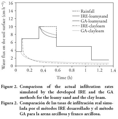
The time when the runoff starts (when the infiltration rate is less than the rainfall rate) calculated using the developed IRE model is 0.349 h for the loamy sand, slightly greater than 0.333 h calculated by the Green Ampt (GA) model (Green and Ampt, 1911; Chu and Mariño, 2005) (Figure 2). The difference in infiltration rate between the GA and IRE methods is within the period of 0.333 h to 0.583 h, and the calculated infiltration rate by the IRE is smaller than that of the GA for the most time of this period. Except for this period of the highest rainfall, the loamy sand infiltrability is large enough to infiltrate all the rainfall. For the clay loam, the runoff starts at 0.07 h according to the GA method. Likewise, the value is 0.095 h for the IRE method. After 0.095 h, the infiltrability is constantly less than rainfall rate.
The calculated cumulative infiltration amount of the two soils using different methods is close to each other (Figure 3). For the loamy sand, the simulated cumulative infiltration by the developed IRE model is 6.5 % and 2.0 % less than those from the FEM method and the GA method, while the cumulative infiltration amount calculated by the IRE method is 13.1 % larger and 13.0 % less than those from the FEM method and the GA method for the clay loam, respectively. Water drainage at the lower boundary is insignificant, because the infiltration water doesn't reach the lower boundary in such a short time.

Figure 4 compares soil water content distribution from the three models at the end of simulation. It is obvious that the calculated water content distribution down the profile using the IRE method is similar with that from the FEM method, more realistic than that from the GA model where sudden changes in soil water content occur. In this case, θs is identical for both loamy sand and clay loam, indicating pore sizes are the same for both soils. For the clay loam, it has the smaller hydraulic conductivity and is easier to get saturated near the upper boundary in soil column.

Case 2: Evaporation experiment
Figure 5 compares the actual evaporation rates simulated by the Yanful's model (Yanful and Mousavi, 2003), the FEM method and the developed IRE method in the study together with the experimental data. For the coarse sand (Figure 5A), the falling evaporation rate starts experimentally on the 5th day, compared to the 6th day by the developed IRE model and the 9th day by the Yanful's model. Clearly, the IRE model gives a better prediction of the date of falling evaporation rate than the Yanful's model. Before the 10th day, the simulated actual evaporation from the Yanful and IRE methods is greater than the experimental value, while opposite is the case for the rest of the simulation period. For the fine sand (Figure 5B), the experimental falling evaporation rate starts at the 6th day, while the 4th and 8th day are simulated by the IRE model and the Yanful's model. The evaporation rate curve produced by the IRE is similar with that by the FEM method. For the coarse sand, the IRE over-predicts the cumulative evaporation by 13.8 %, compared to 17.6 % by the Yanful method, whilst the under-prediction of 15.0 % is simulated for the fine sand by the IRE method, compared with the experimental values. From the above it can be concluded that the developed IRE method performed satisfactorily, compared with the results from the FEM method and the Yanful method.
Case 3: Field experiment
Both the infiltration model and the evaporation model cannot simply be applied due to the interactive processes involved. Therefore, only the FEM method is used for comparing the IRE method with other alternatives. Both the infiltration amounts from the IRE method and the FEM method are 37.4 cm, equal to the cumulative rainfall. This means that all the potential rainfall infiltrated to the soil column. The actual evaporation simulated by the FEM method is less than that of IRE method, whereas the drainage is opposite. However, the cumulative outflow (equal to the amount of evaporation and drainage) simulated by the FEM method is 37.16 cm, slightly more than 35.95 cm simulated by the IRE model.
Figure 6 presents the measured and simulated water content distribution by the IRE and FEM methods at different time intervals. Generally, the results from the IRE model are close to these from the FEM method and the measurements, especially on the 229th, 301th and 319th day. The differences between the IRE and the FEM are mainly in the top 6 cm soil. This might be attributed to the rapid change in the moisture diffusivity during the wet period of the soil. Nevertheless, the results obtained from the developed IRE method are acceptable for practice use.
CONCLUSIONS
A model based on the IRE method was developed in this study for soil water movement modeling in the soil-atmosphere system. The model is much simpler than the FEM method, it is as easy as cascade model to implement, and also achieves accurate results similar to those from the FEM method. The model is able to simulate infiltration into uniform soil with arbitrary initial moisture distributions under an unsteady rainfall event and evaporation as well. Results show the developed model worked well for different soils under different atmospheric conditions and, therefore, the model has the potential to be employed for agro-hydrological simulations in a wide range of fields.
ACKNOWLEDGEMENTS
The work was funded by 973 Program (No. 2013CB227904), the National Natural Science Foundation of China (Nos. U1361214, 51379187), and the Fundamental Research Funds for the Central Universities (No. 2012QNB10). The authors gratefully thank Dr. J. Simunek for providing the SWMS_2D source code, and other experts for providing the validation data in their related studies.
LITERATURE CITED
Agricultural Research Service. 1963. Hydrological data for experimental watersheds in the United States 1956-59. U.S. Department of Agriculture, Washington, D.C. Misc. Publ 945, pp: 62.9-1-62.9-8. [ Links ]
Allen, R. G., L. S. Pereira, D. Raes, and M. Smith. 1998. FAO Irrigation and Drainage Paper No. 56, Crop Evapotranspiration (Guidelines for computing crop water requirements), pp: 15-86. [ Links ]
Aydin, M. 2008. A model for evaporation and drainage investigations at ground of ordinary rainfed-areas. Ecol. Model. 217: 148-156. [ Links ]
Brooks, R. H., and A. T. Corey. 1964. Hydraulic properties of porous media. Hydrol. Paper 3, Civil Engineering Department, Colorado State University, Fort Collins, USA, pp: 1-27. [ Links ]
Burns, I. G. 1974. A model for predicting the redistribution of salts applied to fallow soils after excess rainfall or evaporation. J. Soil Sci. 25: 165-178. [ Links ]
Chu, X., and M. A. Mariño. 2005. Determination of ponding condition and infiltration into layered soils under unsteady rainfall. J. Hydrol. 313: 195-207. [ Links ]
Chu, X. F. 2006. HYDROL-INF Modelling System Version 2.22 User's Manual. [ Links ]
Chu, X., and M. A. Mariño. 2006. Simulation of Infiltration and Surface Runoff, A Windows-Based Hydrologic Modeling System HYDROL-INF. World Environmental and Water Resource Congress 2006, ASCE, 1-8. [ Links ]
Chu, S. T. 1978. Infiltration during an unsteady rain. Water Resour. Res. 14(3): 461-466. [ Links ]
Cook, F. J., and D. W. Rassam. 2002. An analytical model for predicting water table dynamics during drainage and evaporation. J. Hydrol. 263: 105-113. [ Links ]
Gardner, W. R., and D. I. Hillel. 1962. The relation of external evaporation conditions to the drying of soils. J. Geo. Res. Atm. 67: 4319-4325. [ Links ]
Gencoglan, C., S. Gencoglan, H. Merdun, and K. Ucan. 2005. Determination of ponding time and number of on-off cycles for sprinkler irrigation applications. Agr. Water Manage. 72: 47-58. [ Links ]
Green, R. E., and G. A. Ampt. 1911. Studies on soil physics: I. Flow of air and water through soils. J. Agr. Sci. 4: 1-24. [ Links ]
Idso, S. B., R. J. Reginato, and R. D. Jackson. 1979. Calculation of evaporation during the three stages of soil drying. Water Resour. Res. 15: 487-488. [ Links ]
Jain, A., and A. Kumar. 2006. An evaluation of artificial neural network technique for the determination of infiltration model parameters. Appl. Soft. Comput. 6: 272-282. [ Links ]
Jarvis, N., A. Etana, and F. Stagnitti. 2008. Water repellency, near-saturated infiltration and preferential solute transport in a macroporous clay soil. Geoderma. 143: 223-230. [ Links ]
Kay, A. L., and H. N. Davies. 2008. Calculating potential evaporation from climate model data: A source of uncertainty for hydrological climate change impacts. J. Hydrol. 358: 212-239. [ Links ]
Lee, D. H., and L. M. Abriola. 1999. Use of the Richards equation in land surface parameterizations. J. Geophys. Res. 104: 27519-27526. [ Links ]
Lugomela, G. V. 2007. Two-phase flow numerical simulation of infiltration and groundwater drainage in a rice field. Phys. Chem. Earth. 32: 1023-1031. [ Links ]
Miller, E. E., and R. D. Miller. 1956. Physical theory for capillary flow phenomena. J. Appl. Phys. 27: 324-332. [ Links ]
Mollerup, M. 2007. Philip's infiltration equation for variable-head ponded infiltration. J. Hydrol. 347: 173-176. [ Links ]
Parlange, J. Y., R. Haverkamp, and J. Touma. 1985. Infiltration under ponded conditions: 1 optimal analytical solution and comparison with experimental observations. Soil Sci. 139: 305-311. [ Links ]
Peters, A., and W. Durner. 2008. Simplified evaporation method for determining soil hydraulic properties. J. Hydrol. 356: 147-162. [ Links ]
Pielke, R. A., W. R. Cotton, R. L. Walko, C. J. Tremback, W. A. Lyons, L. D. Grasso, M. E. Nicholls, M. D. Moran, D. A. Wesley, T. J. Lee, and J. H. Copeland. 1992. A comprehensive meteorological modeling system-RAMS. Meteorol. Atmos. Phys. 49: 69-91. [ Links ]
Pierson, F. B., P. R. Robichaud, C. A. Moffet, K. E. Spaeth, C. J. Williams, S. P. Hardegree, and P. E. Clark. 2008. Soil water repellency and infiltration in coarse-textured soils of burned and unburned sagebrush ecosystems. Catena 74: 98-108. [ Links ]
Qi, X., X. Zhang, and H. Pang. 2008. An efficient multiple-dimensional finite element solute for water flow in variably saturated soils. Agr. Sci. China. 7: 200-209. [ Links ]
Simunek, J., T. Vogel, and M. Th. van Genuchten. 1994. The SWMS-2D Code for Simulating Water Flow and Solute Transport in Two-Dimensional Variably-Saturated Media, Version 1.21. [ Links ]
Simunek, J., T. Vogel, and M. Th. van Genuchten. 1995. The SWMS-3D Code for Simulating Water Flow and Solute Transport in Three-Dimensional Variably-Saturated Media, Version 1.0. [ Links ]
Somma, F., and J. W. Hopmans. 1998. Transient three-dimensional modeling of soil water and solute transport with simultaneous root growth, root water and nutrient uptake. Plant Soil. 202: 281-293. [ Links ]
Tanny, J., S. Cohen, S. Assouline, F. Lange, A. Grava, D. Berger, B. Teltch, and M. B. Parlange . 2008. Evaporation from a small water reservoir: Direct measurements and estimates. J. Hydrol. 351: 218-229. [ Links ]
Van Genutchten, M. Th. 1980. A closed form equation for predicting the hydraulic conductivity of unsaturated soil. Soil Sci. Soc. Am. J. 44: 892-898. [ Links ]
Van Genutchten, M. Th., F. J. Leij, and S. R. Yates. 1991. The RETC Code for Quantifying the Hydraulic Functions of Unsaturated Soils. EPA. 117 p. [ Links ]
Yanful, E. K., and L. P. Choo. 1997. Measurement of evaporative fluxes from candidate cover soils. Can. Geotech. J. 34: 447-459. [ Links ]
Yanful, E. K., and S. M. Mousavi. 2003. Estimating falling rate evaporation from finite soil columns. Sci. Total Environ. 313: 141-152. [ Links ]
Yang, D., T. Zhang, K. Zhang, D. J. Greenwood, J. P. Hammond, and P. J. White. 2009. An easily implemented agro-hydrological procedure with dynamic root simulation for water transfer in the crop-soil system: Validation and application. J. Hydrol. 370: 177-190. [ Links ]
Zhang, K., T. Zhang, and D. Yang. 2010. An explicit hydrological algorithm for basic flow and transport equations and its application in agro-hydrological models for water and nitrogen dynamics. Agr. Water Manage. 98: 114-123. [ Links ]
Zhang, X., C. Ji, and X. Yuan. 2008. Prediction method for evaporation heat transfer of non-azeotropic refrigerant mixtures flowing inside internally grooved tubes. Appl. Therm. Eng. 28: 1974-1983. [ Links ]

