


Serviços Personalizados
Journal
Artigo
 Inglês (pdf)
 Artigo em XML
 Referências do artigo
 Enviar este artigo por email
Indicadores
-
 Citado por SciELO
 -
 Acessos
Links relacionados
-
 Similares em
SciELO
Similares em
SciELO
Compartilhar

 Permalink
Agrociencia
versão On-line ISSN 2521-9766versão impressa ISSN 1405-3195
Agrociencia vol.43 no.2 Texcoco Fev./Mar. 2009
Agua–suelo–clima
A calibrated agricultural water demand model for three regions in northern Baja California
Un modelo calibrado de demanda de agua para uso agrícola para tres regiones en el norte de Baja California
Josué Medellín–Azuara1* , Richard E. Howitt2 , Cynthia Waller–Barrera3, Leopoldo G. Mendoza–Espinosa3 , Jay R. Lund1, Joseph E. Taylor2
1 Department of Civil and Environmental Engineering. *Author for correspondence: (josuemedellin@gmail.com), (jrlund@ucdavis.edu).
2 Agricultural and Resource Economics. University of California, Davis, One Shields Avenue Davis, CA, 95616 USA. (rehowitt@ucdavis.edu), (jetaylor@ucdavis.edu).
3 Instituto de Investigaciones Oceanológicas. Universidad Autónoma de Baja California. Km. 107 Carretera Ensenada–Tijuana, Ensenada, Baja California, México (lmendoza@uabc.mx).
Received: February, 2008.
Aproved: January, 2009.
Abstract
Irrigated agriculture is the largest water user in many regions, and agricultural water use efficiency and consumption has been studied by several authors. This paper provides a framework and application of economic valuation of water for agriculture in three regions in northern Baja California, Mexico, namely Guadalupe, Maneadero and Mexicali Valleys. Positive mathematical programming (PMP), a deductive valuation technique, was the framework used for this estimation using water delivery data reported by the National Water Commission in Mexicali, production costs and cultivated area, production factors use from the Agriculture Ministry (SAGARPA); and other data from previous studies. Analysis of the results shows that marginal economic water value in Mexicali is at least 2.6 times the water price paid by farmers. Guadalupe and Maneadero with higher value agriculture, have higher marginal economic values of water than Mexicali, albeit closer to their water costs. Small shortages increase this economic value for farmers. Estimated price elasticities of irrigation water for each turn–out are inelastic for all regions and within the range of most previous studies. Policies aimed to reduce water consumption by decreasing current pumping subsidies are encouraged.
Key words: Mathematical programming, Baja California, economic water valuation.
Resumen
La agricultura de riego es la actividad que más agua usa en muchas regiones, y la eficiencia y consumo del uso agrícola del agua ha sido estudiada por varios autores. Este estudio provee un marco conceptual y la aplicación de la valoración económica del agua para uso agrícola en tres regiones del norte de Baja California, México, a saber, los valles de Guadalupe, Maneadero y Mexicali. El marco de referencia usado para esta estimación fue la programación matemática positiva (PMP), una técnica de valoración deductiva usando datos del suministro de agua reportados por la Comisión Nacional del Agua en Mexicali, costos de producción y área cultivada, uso de factores de producción de la Secretaría de Agricultura (SAGARPA), y otros datos de estudios anteriores. El análisis de los resultados muestra que el valor económico marginal del agua en Mexicali es al menos 2.6 veces el precio del agua que pagan los agricultores. Guadalupe y Maneadero, que tienen un mayor valor de producción agrícola, tienen valores económicos marginales del agua mayores que Mexicali, aunque más cercanos a sus costos de agua. Pequeños déficits de agua aumentan este valor económico para los agricultores. Las elasticidades precio del agua estimadas para irrigación de cada resultado son inelásticas para todas las regiones y dentro del rango de la mayoría de los estudios previos. Se recomiendan las políticas dirigidas a reducir el consumo de agua al disminuir los subsidios actuales para la extracción.
Palabras clave: Programación matemática, Baja California, valoración económica del agua.
INTRODUCTION
Estimating economic water demand for irrigation has increasing importance for both policymakers and stakeholders. Without knowing the economic value of irrigation water use, water pricing policies can give inappropriate incentives and foster overexploitation of the resource (Tsur et al., 2004). In this paper the economic value of water for irrigation in Baja California, México, is estimated and discussed using an empirically calibrated deductive valuation technique called positive mathematical programming or PMP (Howitt, 1995). In this setting, farms or groups of similar farms use irrigation water to maximize profit. For profit–seeking farmers, the marginal economic value of water use exceeds the current water cost. This application of PMP extends the Statewide Wide Agricultural Production model (SWAP) for USA, California. SWAP is used to provide economic penalty functions for the California–wide hydro–economic model CALVIN (Jenkins et al., 2004).
The agricultural regions of Guadalupe, Maneadero and Mexicali are presented as case studies, using data on water deliveries. This application of PMP offers improvements over previous models used in México (Florencio–Cruz et al., 2002; Howitt and Medellín–Azuara, 2008; Tsur et al., 2004), with a less restrictive production function and greater spatial disaggregation. Results contrast agricultural water value among these three agricultural regions. The irrigation delivery valuation model developed here supports the more recent hydro–economic model Baja CALVIN[4].
Irrigation water valuation techniques
Economic valuation of irrigation water has been studied since the 1960s (e.g. Moore and Hedges, 1963). In inductive approaches water is a variable input, whereas in the deductive approaches water is hypothesized as a limiting factor (Young, 2005). New approaches using generalized maximum entropy claim to establish a continuum between those two broad valuation categories (Heckelei and Wolff, 2003).
In a meta–analysis of irrigation water demand literature, Scheierling et al. (2006) found that price–elasticities of demand for irrigation water averaged –0.48 with a median of –0.16, both in the inelastic range. Compared to inductive techniques, deductive techniques have been reported to give higher estimates of economic water value (Scheierling et al., 2006; Young, 2005). The deductive PMP technique (Howitt, 1995), used in this study, has several advantages over traditional econometric (inductive) methods to estimate economic values of water. First, the PMP cost function calibrates exactly to observed values of production output and factor use, which provides a more deductive and production–theoretic model structure. Second, PMP adds flexibility to the profit function by relaxing the restrictive linear cost assumption. Finally, PMP does not require large datasets as many econometric methods, and thus enables price variability among disaggregated estimates.
MATERIALS AND METHODS
PMP is a self–calibrating three–step procedure (Howitt, 1995). First, a linear program for profit maximization is solved. In addition to traditional resource and non–negativity constraints, calibration constraints restrict land use and crop mix to observed values. The second step solves for the parameters of a quadratic cost function using Lagrange multipliers from calibration constraints from the first step, and the production function from first order conditions. Derivations and mathematical formulations of these parameters are presented in Medellín–Azuara et al. (2007). The third step incorporates the recently calibrated functions into a non–linear profit maximization program, with constraints on resource use. Economic values of water are obtained by restricting water availability for each region. A multi–region and multi–crop program, for a profit maximizing representative farmer, is assumed for each crop and group of farms. Heterogeneity in production is addressed for both crops and farm groups. The unit of analysis is a group of farm producers with similar production characteristics in a region.
The production function is represented by the Constant Elasticity of Substitution (CES) functional form shown in equation (1):
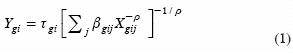
where sub–index g corresponds to the agricultural region, i refers to crop type, and j to production factors or inputs. The model inputs are land, labor, water and supplies. Ygi is the output for crop i in region or group g. The scale parameter of the CES production function is τgi, and share parameters for the resources for each crop are given by βgi. The decision variable Xgij denotes use of factor j in production of crop i of region g. The elasticity of substitution σ is given by σ = 1/(1 + ρ). For this model, the elasticity of substitution is the same for all crops and all farm groups.
First step: linear program
The linear program with calibration constraints is as follows:
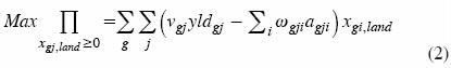
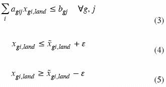
Equation (2) is the objective function. Decision variables are xgi,land , planted hectares for region or group g and crop i. The marginal revenue of crop i in region g is vgi . Average yields and average variable costs are given by yldgi and ωgi. Leontief coefficients agji are given by the ratio of total input usage to land. For this step, production inputs are normalized to land.
The resource constraint is given by (3), in which production factors j are limited by the parameter bgi in every region. Sets (4) and (5) represent upper and lower bounds of calibration, and the  is the observed value of resources usage, whereas ε is a small tolerance for decoupling.
Second step: parameterization of a non–linear cost function
The cost function is given by (6):
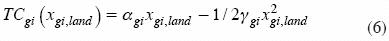
where αgi and γgi are the intercept and the slope of a linear marginal cost function for crop i in region g. Since average costs ωgi in the objective function (2) are variable, and assuming marginal revenue equals marginal cost,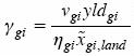 where ηgi is the price–elasticity of supply for crop i in region g. Average cost is given by
 and i, where ACgi =
  and i, where λ2,gi,land is the dual value of the binding calibration constraints set in (4) and (5).
Third step: non–linear program
This step is to solve a non–linear constrained profit maximization program. The objective function is:
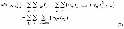
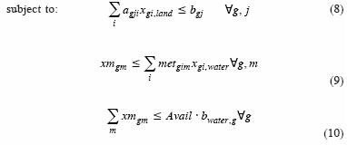
Ygi is defined by the production function in equation (1) with parameters τgi and βgij derived in Medellín–Azuara et al., (2007). The second term is the PMP calibrated cost function. Constraint set (8) is as in (3) with all J resources (not just subset K). A new constraint set on monthly water use is included. Variable xmgm in (9) is monthly water use in region g in month m.
Three underlying assumptions are worth discussing. First, water is interchangeable among crops within a region. Second, a farm group (or region) maximizes annual profits and water is allocated across the growing season to equalize its monthly marginal products. Third, a region picks the crop mix that maximizes profits. This assumes sufficient water storage and internal water distribution capacity. In constraint set (10) bwater,g corresponds to bgi for water in 98(8). The parameter Availg is used to obtain shadow values of water by varying O<Availg < 1.Constraint set (10) assumes that yearly water is available in a limited amount for every region or group. Less realistically, it also implies that water is not re–traded across groups or regions under the basic calibration assumptions.
Dataset for the Positive Mathematical Programming application
The model requires several datasets on planted hectares, factor usage, and market prices of products and factors in the study region. Datasets for this model were assembled using data from SAGARPA (2006) for Guadalupe and Maneadero and previous work by Medellín–Azuara et al. (2007) for Mexicali from digital sources and reports from SAGARPA, CNA and Baja California State agencies. Production factors were land, water, labor and supplies.
For 2000 to 2005, the Agriculture Ministry (SAGARPA[5]) database provides information on planted land by crop, yields, mean rural price, and production value by municipality. CNA water delivery reports in Irrigation District 014 (ID 014) complemented the database.
The municipality of Mexicali covers most of ID 014. Part of ID 014 is in San Luis Río Colorado, Sonora. The valleys of Guadalupe and Maneadero, in the Ensenada subregion, rely entirely on groundwater and are composites of irrigation units. In Guadalupe, from 28 to 32 million cubic meters (Mm ) of water are extracted yearly from the Guadalupe aquifer. About a third of this water is for urban uses in Ensenada and the rest for agriculture (Daesslé et al., 2006).
Cost and production information for the Guadalupe and Maneadero was provided by the regional offices of SAGARPA and CNA. Three years of observations on cultivated land, yields, water, labor, supplies and prices were used. The crop mix in each region is summarized in Table 1. The crop mixes for both agricultural regions account for roughly 82 % of the total water use, so regional water demand functions have to be scaled up to represent total use. The rationale for this assumption is that the highest productive uses of water are well represented by the available crop mixes and should not be part of the remaining 18% of water.
Selection of representative crops in Guadalupe and Maneadero
The crops (Table 1) amount to slightly more than 80% of total production, cultivated surface and water consumption. Water consumption was calculated using average water surface applications for each crop and its cultivated surface. Average production costs for Maneadero and Guadalupe are included for 2002–2004. Green onion, vine tomato, flowers and organic tomato have the highest average production costs. Labor required by each type of crop is also included. Labor cost for 2002 and 2003 was US $9.1 d–1 and US $10.0 d–1 for the year 2004 for both agricultural areas. Water extraction cost averaged $0.14 US m–3 from SAGARPA, including energy for pumping.
Cumulative values (2004) for the representative crops in each Ensenada region are shown in Tables 2 and 3. For Maneadero, tomatoes cover the most area, followed by olive trees and flowers. Tomatoes provide by far the largest production volume, followed by flowers and onions. Tomatoes have the largest production value, followed by peas and flowers.
Production costs for Guadalupe and Maneadero
Variable costs for Guadalupe and Maneadero were calculated using SAGARPA data on costs of soil preparation, sowing, harvest, pesticide application, technical assistance, etc. This information was used to calculate, according to labor, cost per hectare and supply cost per hectare for each crop. The estimated yearly land rental cost, provided by SAGARPA staff, varied between $1500 and $1200 dollars ha–1 for Guadalupe and Maneadero.
Crop mix and costs for Mexicali
The crop mix selected for Mexicali was based on the proportion of total cultivated land (Medellín–Azuara et al., 2007). Water years 2000–2005 had estimated water deliveries. The crop mix for Mexicali (Table 4) covered 182 030 irrigated ha in 2005 (CNA, 2006) and a volume of 1982 MCM yr–1. In Table 4 it is shown that crop mix covers roughly 85 % of the cultivated land and slightly more than 83 % of the water delivered for Mexicali Valley irrigation. Most land and water use data is from the Office of Statistics of Irrigation District 014, through their annual Water Use Report or Informes de Distribución de Aguas. Electronic databases provided information on planted hectares, and monthly water deliveries per crop group and module and water source (surface or groundwater). Monthly water deliveries establish a seasonal water use pattern for the Mexicali valley for each irrigation module.
Factor use and cost information were available from the ID 014, the state office of SAGARPA, and a study on the All American Canal lining (Sosa–Gordillo and Sánchez–López, 2007). Average production costs and mean rural product prices were available for some water years from 2000–2005. Detailed cost information was available only for some crops; however, data for the crop mix for our study (Table 4) was reasonably consistent among state and federal agencies including mean rural prices for the crop output in the base year (SAGARPA, 2006).
The Mean Rural Price for Mexicali and factor usage are summarized in Table 5. Labor is as in Table 1. Water price from 2001 to 2005 averaged US $7.00/1000 m3 in Mexicali. Supplies costs (not itemized) are an aggregation of the remaining variable costs. These were approximated from the SAGARPA's total variable cost not related to water, labor or land rental.
The 22 modules for the Mexicali Valley were aggregated into four groups based on geographical location, land quality and primary water sources. The groups were named, East of the Colorado River, Main Valley, West Valley and Groundwater. Details on module aggregation appear in Medellín–Azuara et al. (2007). The East group modules are in the state of Sonora. The economic value of water for this group is expected to be higher than average for the district, with high value crops such as asparagus and green onion.
A second group of modules has higher use of groundwater, including modules near the USA–Mexico border with Arizona where at least 22 % of their crop area is cotton. Wheat is the most common crop in ID 014 in terms of land share, but the groundwater group has less than the district's average of 56 %.
The Main Valley group contains seven modules which make higher use of surface water, for alfalfa and wheat. Asparagus and green onion are less common in this group. Finally, the West side group has lower value crops, relative water surplus, a higher share of lower quality land, and are usually considered water sellers. Cultivated land follows about the same pattern as for the Main Valley group and even higher value crops have more area than in the center of the valley. Forages are next in importance after the three main crops.
RESULTS AND DISCUSSION
To obtain economic marginal values of water for each location, water availability was reduced from 100 % to 60 % in ten percent steps. The water availability constraint (10) is regional, permitting transfers of water among crops within a region. It is assumed that marginal revenue product of the optimized crop mix equals its marginal cost. The programs and parameters in equations (1) to (10) were solved using GAMSTM (General Algebraic Modeling System, 2008).
Calibration of the model to observed values occurred in the first and third steps. The criteria were first, difference in input use and second, difference in output for all regions and all crops with respect to observed values. In most cases the percent difference of input use was on the order of 10–6, for both stages.
Model results for Guadalupe and Maneadero
SWAP results provide economic value of agricultural water use in Guadalupe and Maneadero. In Figure 1 it is shown the marginal economic value of water, that is what the farmer is willing to pay for having an additional thousand cubic meters of water at each availability level. Although applied water varies by month, the model assumes similar marginal values of water across months due to profit–maximizing behavior by farmers.
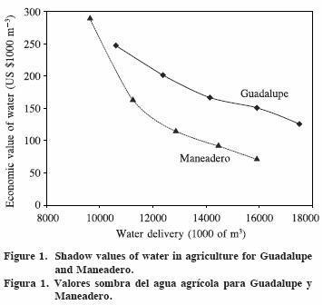
At current water availability, the shadow values of water for agricultural uses in Guadalupe and Maneadero are 72 and 126 dollars per thousand cubic meters ($US1000 m–3). With water shortages of 60 %, this shadow value increases to 290 $US1000 m–3. The Maneadero shadow value compares to that of some irrigation subdistricts in the Mexicali Valley (see below). However, the shadow value of water for Guadalupe is consistently higher.
Economic values in Maneadero span a wider water range than that for Guadalupe because Maneadero has a larger price–elasticity of demand for water at all levels of delivered water studied. Average price elasticies are –0.56 and –0.31, within the range of Scheierling et al. (2006) meta–analysis for irrigation water demand. At 100 % of current water availability in Guadalupe, marginal economic value of water is US $126 1000 m–3, roughly the average pumping cost. With a 20 % shortage, the willingness to pay for additional water increases about 1.3 times.
Results for Mexicali
For Mexicali, results of the water availability parametric runs appear in Figure 2. Overall, agriculture in the West of the Mexicali Valley has the lowest shadow value of irrigation water when availability drops below 80 %. The Main Valley group has the highest economic values whereas the East side keeps the same value just in the average of the four regions. Groundwater follows a steepest pattern in Figure 2, beginning as the lowest water value at current availability and passing valuation in other two regions at the lowest level of availability.
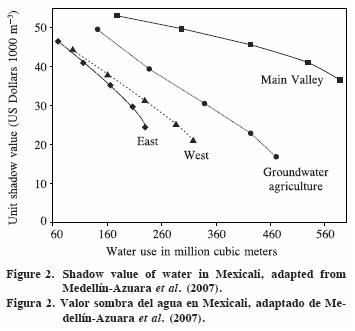
Also compares annual regional water demands were also compared (Figure 2). The shadow value of water is the lowest at full availability for groundwater agriculture. A value of 16.9 US $1000 m–3 is 2.67 times the fee paid for 2005 of 6.27 US $1000 m–3 (CNA, 2005). Officials at ID 014 indicated that market price for water is about $65 US $ ha–1. Currently, a hectare has an average allocation of about 100 cm which yields 10 000 m–3, resulting in a price of US $6.4 1000 m–3. Thus, apparently the spot market price for water is similar to the water fee paid. Extreme conditions of scarcity (60 %) increase the ratio of current value to price from 2.67 to 7.86, the second highest of the four regions. An argument for such a drastic change in water value relative to other regions is that water use intensity (as volume per hectare) is higher due to water intense crops. However, group has the highest yield factor of 1.16 (Medellín–Azuara et al., 2007). As water becomes scarce, the high marginal product of water for this high–yield group increases the shadow value more relative to other regions.
East side agriculture economic value of water is surprising, with shadow values roughly the average of the valley at all levels of availability. One explanation is that a large module within the East group has a high proportion of low quality soils. This may ultimately affect water valuation with greater scarcity. Valuation of waters in Main Valley agriculture is higher than expected, as highly subsidized crops such as alfalfa, wheat and cotton are well represented.
Finally, West side agriculture is likely to sell water to other regions or urban uses. Low value crops and poor quality land reduce the marginal product of water. However, this does not seem to be the case for water scarcities below 20 %, for which the groundwater region would seem a better candidate to sell water. This is unlikely. Historically, regions close to the Colorado River purchase supplemental water for irrigation (Medellín–Azuara et al., 2007). One explanation for this erratic behavior is that price–elasticity of supply (ηgi) is assumed to be the same for all crops and all regions. As better information on this parameter is obtained from econometric studies in the valley, a better response estimate would be obtained. Regions with a higher value crop mix would respond more drastically to even small shortages.
Medellín–Azuara et al. (2007) indicated that water price elasticity in the Mexicali Valley ranged from –0.50 for conditions of relative abundance, to –0.66 at 60 % water availability. Estimated price–elasticities seem to fall within the range of most values at observed levels of production (Scheierling et al., 2006). For irrigation with groundwater, reducing pumping subsidies may decrease overpumping and increase the marginal economic value of water.
Model limitations and extensions
Some limitations of this model are reviewed here and detailed by Medellín–Azuara et al. (2007). Disaggregated production models usually require more time and data. However, they have proved to be effective in modeling with higher precision policy changes in some rural economies (Taylor et al., 2005). The underlying assumption is that farmer reactions within an agricultural region are similar. Although there will often be small and large agricultural production units. The Guadalupe, Maneadero, and Mexicali areas are commercial agriculture with commercial reasons for farmers to behave similarly.
Data limitations on production costs present difficulties for economic water value estimates, as average costs are used for Ensenada and Mexicali. This is not a problem for costs that remain more or less static and homogeneous for all users such as water and labor costs. Land rental prices are mostly based on land quality characteristics. Nevertheless, supplies and resource use may vary from farmer to farmer depending on particular characteristics of the production units. Furthermore, consolidating land use and cost information from different agencies may introduce some bias in the economic marginal value estimations. In general, underestimated costs or factors usage may produce higher marginal economic values of water. One of the advantages of these models is that these concerns can be addressed easily as more data becomes available. Hopefully, the availability of models of this type will motivate development of better data.
CONCLUSIONS
This paper offers a method to estimate economic water demand and value for irrigation even with minimum datasets. The Baja California regions of Guadalupe, Maneadero and Mexicali offer an excellent case study to value water in irrigated agriculture. This uniqueness is characterized by the absence of rain–fed agriculture, a relatively homogenous topography, a high proportion of high quality soils, and in the case of Mexicali, a lower bound for water availability.
The ratio of the marginal economic value to the water fee for current water supply conditions ranged from 1.3 to 5.9. The estimated price–elasticity of irrigation water falls within the average reported by meta–analysis literature on the field. Low–value crops, or those in poor–land quality agricultural regions are the likely sellers of water with increasing water scarcity. However, water pricing policies alone without markets, other rationing, or restrictions on sales could lead to unintended and undesirable income distribution effects.
Finally, results using mathematical programming techniques call for caution on interpretation of results, as some omitted costs may decrease water marginal economic value. The same would occur if water use from the base dataset is underestimated. Thus, marginal economic value estimations from this study can be taken as a solid average upper bound for irrigation water value in Baja California.
AKNOWLEDGEMENTS
We are thankful for funding provided by CONACYT–UCMEXUS and the California Environmental Protection Agency (CALEPA). We are indebted to agencies and institutions that provided data: CNA, SAGARPA and UABC–Mexicali.
LITERATURE CITED
CNA (Comisión Nacional del Agua). 2005. Reporte Histórico de Ingresos. Jefatura del Distrito de Riego 014. Mexicali, México. CD–ROM. [ Links ]
CNA (Comisión Nacional del Agua). 2006. Informes de Distribución de Aguas 2000–2006. Anexos II. Jefatura del Distrito de Riego 014, Río Colorado, Mexicali, Baja California, México. CD–ROM. [ Links ]
Daesslé, L. W., L. G. Mendoza–Espinosa, V. F. Camacho–Ibar, W. Rozier, O. Morton, L. Van Dorso, K. C. Lugo–Ibarra, A. L. Quintanilla–Montoya and A. Rodríguez–Pinal. 2006. The hydrogeochemistry of a heavily used aquifer in the Mexican wine–producing Guadalupe Valley, Baja California. Environ. Geol. 51: 151–159. [ Links ]
Florencio–Cruz, V., R. Valdivia–Alcalá, and C. A. Scott. 2002. Water productivity in the Alto Rio Lerma (011) Irrigation District. Agrociencia 36(4): 483–493. [ Links ]
Heckelei, T., and H. Wolff. 2003. Estimation of constrained optimisation models for agricultural supply analysis based on generalised maximum entropy. European Rev. Agric. Econ. 30(1): 27–50. [ Links ]
Howitt R. E. 1995. "Positive Mathematical Programming". American Journal of Agricultural Economics, 77: 329–342. [ Links ]
Howitt, R. E., and J. Medellín–Azuara. 2008. "Un Modelo Regional Agrícola de Equilibrio Parcial: El Caso de la Cuenca del Río Bravo in Guerrero–García–Rojas, H. R, A. Yúnez–Naude, and J. Medellín–Azuara (eds.) El Agua en México: Consecuencias de las políticas de intervención en el sector. Lecturas El Trimestre Económico 100. Fondo de Cultura Económica. México, D. F. 222 p. [ Links ]
Jenkins, M. W., J. R. Lund, R. E. Howitt, A. J. Draper, S. M. Msangi, S. K. Tanaka, R. S. Ritzema, and G. F. Marques. 2004. "Optimization of California's water supply system: Results and insights." J. Water Resources Planning and Manag.–ASCE 130(4): 271–280. [ Links ]
Medellín–Azuara, J., J. R. Lund, and R. E. Howitt. 2007. "Water Supply Analysis for Restoring the Colorado River Delta, Mexico." J. Water Resources Planning and Manag. 133(5): 462–471. [ Links ]
Moore, C. V., and T. R. Hedges. 1963. A method for estimating the demand for irrigation water. Agric. Econ. Res. 15(4): 131–135. [ Links ]
SAGARPA (Secretaría de Agricultura, Ganadería, Desarrollo Rural, Pesca y Alimentación). 2006. Sistema de Información Agroalimentaria y Pesquera (SIAP), Secretaría de Agricultura, Ganadería, Desarrollo Rural, Pesca y Alimentación. Viewed June 2006 <http://www.siap.sagarpa.gob.mx/> . [ Links ]
Scheierling, S. M., J. B. Loomis, and R. A. Young. 2006. Irrigation water demand: A meta–analysis of price elasticities. Water Resources Res. 42(1), W01411, doi:10.1029/2005WR004009. [ Links ]
Sosa–Gordillo, J. F., and E. Sánchez–López. 2007. Estudio de los efectos socio–económicos en el Valle de Mexicali provocados por el revestimiento del Canal Todo Americano. Revista Mexicana de Agronegocios 21(2): 18. [ Links ]
Taylor, J. E., G. A. Dyer, and A. Yúnez–Naude. 2005. Disaggregated rural economywide models for policy analysis. World Develop. 33(10): 1671–1688. [ Links ]
Tsur, Y., T. Roe, A. Dinar, and M. Doukkali. 2004. Pricing Irrigation Water: Principles and Cases from Developing Countries, Resources for the Future. Washington, D.C. 319 p. [ Links ]
Young, R. A. 2005. Determining the Economic Value of Water: Concepts and Methods, Resources for the Future. Washington, D.C. 374 p. [ Links ]
4 Viewed 31 January 2008. Consultado el 31 de enero, 2008 en: <http://cee.engr.ucdavis.edu/BajaCALVIN> . [ Links ]
5 Viewed 31 January 2008. Consultado el 31 de enero, 2008, en: <http://siap.sagarpa.gob.mx> . [ Links ]

