


 nueva página del texto (beta)
 Inglés (pdf)
 Artículo en XML
 Referencias del artículo
 Enviar artículo por email
 Citado por SciELO
  Similares en
SciELO
Similares en
SciELO 
 Permalink
Introduction
High-elevation forests in México have gained increasing attention due to their vulnerability to climate variability that impacts their species range distribution (Astudillo-Sánchez, Fowler, Villanueva-Díaz, Endara-Agramont y Soria-Díaz, 2019; Rehfeldt, Crookston, Sáenz-Romero y Campbell, 2012), physiological traits (Correa-Díaz, Gómez-Guerrero, Vargas-Hernández, Rozenberg y Horwath, 2020; Gómez-Guerrero, Silva, Barrera-Reyes, Kishchuk, Velazquez-Martinez et al., 2013; Saenz-Romero, Lamy, Loya-Rebollar, Plaza-Aguilar, Burlett et al., 2013), and forest productivity (Correa-Díaz, Silva, Horwath, Gómez-Guerrero, Vargas-Hernández et al., 2019). However, despite their prominent ecological importance (Holtmeier, 2009; Körner, 2012), climatic information at high elevations is often unavailable, which strongly limits any further analysis and interpretation of ecological processes. In México, climatic stations are mainly located at lower elevations or close to human settlements as their distribution was mostly planned for agricultural purposes. Indeed, according to the (National Meteorological Service database of México [SMN] 2020), only 30 of the 5467 climatic stations (0.5%) were established above 3000 m a.s.l. whereas 17 of them have already been suspended.
In this context, other climatic sources have been generated to fulfill the climatic data need. For example, the Climatic Research Unit (CRU) database from the University of East Anglia, has been turned into a regular source of climatic information but with limited local adequacy due to its coarse resolution (0.5° resolution) (Harris, Jones, Osborn y Lister, 2014). Other approaches have relied on downscaling approaches (Mosier, Hill y Sharp, 2014; Wang, Hamann, Spittlehouse y Carroll, 2016) or spline interpolators (Cuervo-Robayo, Téllez-Valdés, Gómez-Albores, Venegas-Barrera, Manjarrez et al., 2014) which allow generating time series at finer resolutions. For example, the use of downscaling approaches through a combination of local interpolations and terrain elevation adjustments has improved the accuracy and the scale of climatic data. Nevertheless, the lack of in situ information produces high uncertainty at mountain regions where the topographic factors temporally and spatially shape the climate (Körner, 2007), making it a challenging task to calibrate models or disentangle the impact of climate change in forest ecosystem functioning.
Currently, some efforts have been made by locating weather stations to record climatic variables in Mexican high-elevation forests (Biondi, Hartsough y Galindo-Estrada, 2009; Biondi, Hartsough y Galindo-Estrada, 2005). However, out of these examples, there are few reports of climatic conditions at high-elevation forests. It is therefore worthy to investigate how the weather varies across time scales (from hourly to a monthly level) and how the topography of the landscape shapes the temperature and relative humidity in alpine ecosystems, and most importantly, how we can verify the correlation of gross climate sources to local instrumental measurements.
Ecological systems are often hierarchically organized, with levels of organization nested within higher levels usually measured across time, thus traditional statistical approaches are unsuitable to analyze variables from these datasets since the observations measured within a higher level (e.g., mountains) are more correlated to observations between levels, violating therefore the independence assumption (Wagner, Hayes y Bremigan, 2006). Linear mixed models (also called hierarchical linear models) include a combination of fixed and random effects as predictor variables, which allow modeling the non-independence and the correlation structure (Everitt, 2005). Fixed effects represent all possible levels of a factor of study for which researchers are interested while random effects typically represent some grouping variable affecting indirectly the main response (Harrison, Donaldson, Correa-Cano, Evans, Fisher et al., 2018). Thus, the fixed effects are used to model the effects of individual levels of a categorical variable on a continuous variable while random effects express additional model variability, which is usually represented by parametrized covariances structures (Ćwiek-Kupczyńska, Filipiak, Markiewicz, Rocca-Serra, Gonzalez-Beltran et al., 2020). In this way, the fixed effects define the expected values of the observations, and random effects define their variance and covariance.
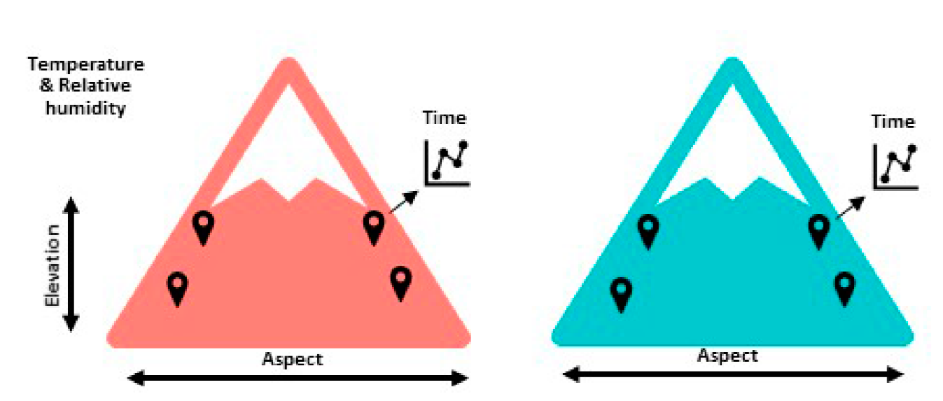
In this work, through linear mixed models we analyzed in situ data of two climatic variables (temperature and relative humidity), gathered at 4-hours intervals from 2016 to 2020, at forests located in separately mountains, namely, Tláloc (TLA) and Jocotitlán (JOC), in the State of México, México. We retrieved climatic data from two contrasting aspects (Northwest and Southwest) across elevation belts (from 3500 m to 3900 m a.s.l.), representing a hierarchical structure for the distribution range of the Mexican Mountain Pine (Pinus hartwegii Lindl.).
Objectives
Our goals were first to evaluate the topographic effect (elevation and aspect) on climatic variables (temperature and relative humidity) and their interannual behavior (hourly and monthly), and second, to compare this instrumental information with data extracted from the ClimateNA software (Wang et al., 2016), a large-scale algorithm which allows a downscaling process using a digital elevation model.
Materials and methods
Study design and dataloggers installation
We studied the climatic conditions in two mountains located across the Trans-Mexican volcanic belt (TLA 19.39° N, -98.74°O, 4125 m a.s.l.; and JOC - 19.72° N, - 99.76°O, 3910 m a.s.l.). At each mountain, we selected two different elevations with contrasting aspects (four sites per mountain). Thus, for TLA, we placed commercial dataloggers (HOBO Pro v2) at 3500 m and 3900 m a.s.l. with contrasting aspects each (Northwest and Southwest), and for JOC at 3700 m and 3800 m a.s.l. using the same aspects that TLA (Fig. 1). These elevations represent the middle and upper (timberline) natural distribution of pure stands of Pinus hartwegii at each mountain. The dataloggers, registering 4-hour intervals of climatic information (temperature and relative humidity), were placed at a high of 2.5 m above the soil level using trees as supports. The HOBO Pro v2 dataloggers have an operation range from - 40 °C to 70 °C and 0% to 100%, with an accuracy of ± 0.21 °C and ± 0.25% for temperature and relative humidity, respectively.
Statistical analysis
We use linear mixed models to test the effect of the mountain origin, elevation, aspect, and time on temperature and relative humidity, using the “nlme” package in R (Pinheiro, Bates, DebRoy, Sarkar y Team, 2018). Conversely to traditional methods, repeated measure data requires special methods of analysis since measurements are often correlated temporally; thus, the linear mixed models allow modeling heterogeneous variance and correlated data.
Our climatic dataset contained three hierarchy levels: the climatic variables (temperature and relative humidity) registered over time (level-1) were selected from eight datalogger locations (level-2) within two mountains (level-3). Therefore, our predictors were time (as hourly and monthly factors) [1], elevation and aspect [2], and finally the mountain origin [3].
Where
𝑌𝑖j = climatic variable (temperature or relative humidity) on the time i in site j and mountain k
𝜎2 = residual variance component due to differences on time within sites nested within mountains
Where:
where:
Thus, the combined model is described in [4].
To achieve linear assumptions in modeling, we transformed our original variables (T and RH) into a new dataset, comparing different transformations and selecting the best one based on the Pearson P test statistic for normality (Gross y Ligges, 2015). We compared the arcsinh, Box-Cox, logarithm, Yeo-Johnson, and ordered quantile normalization (ORQ) transformations using the “bestNormalize” package in R (Peterson y Cavanaugh, 2020).
Furthermore, due to the temporal correlation of the data and the desirable parsimony of the models, different correlation (covariance) structures (autoregressive process - AR, autoregressive moving average process- ARMA, and constant correlation) and variance functions (Power variance and constant variance) were tested to model the correlational structure across time and homogenize the residual variance, respectively (Everitt, 2005). The best model for each variable (T and RH) was defined according to the lowest Akaike Information Criterion (AIC) and Bayesian Information Criterion (BIC), and the highest marginal and conditional R2 (Mehtatalo, 2013). All analyses were done in R 4.03 (R Core Team, 2020) and visualized using the “ggplot” package (Wickham, 2016). We used our climatic data to test the null hypothesis that temperature and relative humidity do not change over time, or across elevations, aspects, or between mountains.
Climatic comparison between sources
For our second objective, we extracted temperature and relative humidity values using the ClimateNA v630 software package for our datalogger locations (Wang et al., 2016; Wang, Hamann, Spittlehouse y Murdock, 2012). ClimateNA allows producing monthly time series at a scale-free level using the climatic database of the University of East Anglia (Harris et al., 2014). Overall, the ClimateNA software uses bilinear interpolations to estimate values between midpoints of the four neighbor grids from a specific location, and thus, generate a surface for each monthly climatic variable. Then, the climate and elevation values from surrounding cells are used to calculate differences between all possible pairs. Finally, a simple linear regression of the differences in the climatic variable on the elevation difference is established, using the slope of the model to predict the climatic value at each specific location (Wang et al., 2016). For comparison purposes, we used a downscaled climatic time series according to a 15-m digital elevation model of our study sites (ClimateNA), and our hourly climatic data was reduced to monthly values. We used the Pearson correlation coefficient (r) between sources and a paired samples t-test to prove that the mean difference between in situ data and the geographical algorithm (ClimateNA) was equal to zero.
Results and discussion
Average temperature and relative humidity at mountain level
A total of 36 930 and 32 411 observations were retrieved from TLA and JOC, respectively, covering from September 2016 to December 2020. Although not all the sites had the maximum span, they covered at least from the 2017 year. At a mountain level, TLA had an average temperature of 7.56 °C ± 0.03 °C while JOC 6.98 °C ± 0.2 °C with significative statistical difference between mountains (p = 0.01). The average temperature was within the expected values for treelines around the world (6.7 °C ± 0.8 °C) (Körner y Paulsen, 2004), but slightly warmer than other Mexican mountains (Nevado de Toluca, Pico de Orizaba, and Iztaccihuatl) (Körner, 2012). The extreme temperatures observed were -6.01 °C and 34.73 °C for TLA, and -7.09 °C and 33.2 °C for JOC, respectively (Fig. 2a). The highest weather station in México (Nevado de Toluca - 4283 m a.s.l.) reported extreme temperatures of -10 °C and 23 °C, while Biondi et al. (2005) at Nevado de Colima (3 760 m a.s.l.) reported -12.7 °C and 18.2 °C, but notably, none of them reached our maximum temperature values. Trees growing at alpine ecosystems have acquired a remarkable frost tolerance during winter; for example, some trees from the genus of Abies and Pinus can tolerate temperatures around -35 °C (Holtmeier, 2009) but higher temperatures can have serious implications for water stress and photosynthetic activity at treeline zones (Hoch y Korner, 2003).
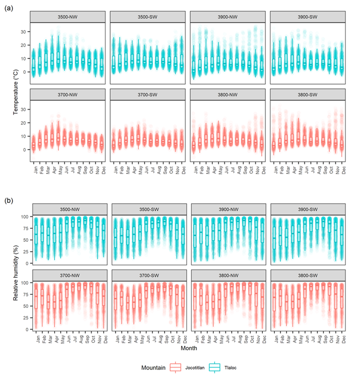
Figure 2 Monthly boxplots of (a) temperature and (b) relative humidity displaying five statistics (the median, two hinges, and two whiskers).
The lower and upper hinges correspond to the first and third quartiles while the lower and upper whiskers extend from the hinge to the smallest/largest value at 1.5 of interquartile range. The datalogger locations (sites) are defined as a combination of elevation (3500 m, 3700 m, 3800 m, and 3900 m a.s.l.) and aspect (Northwest - NW, and Southwest - SW) within each Mountain.
For relative humidity, JOC had a higher average relative humidity than TLA (72.5% ± 0.12% vs 69.30% ± 0.13%, respectively) (p = 0.01), values similar for those reported by Biondi et al. (2005) at Nevado de Colima (69% annual average). Although these differences in relative humidity seem to be small, the differences in terms of water vapor pressure are higher. Usually, alpine forests showed high values of relative humidity due to cloudy conditions and that lower temperatures can retain less humidity than the warmer air (Fig. 2b).
The monthly, daily, and hourly trends
At a monthly level, May was the warmest month for TLA and JOC (9.61 °C ± 0.10 °C and 9.39 °C ± 0.08 °C for average temperature, respectively), when cloud-free conditions occur (Fig. 2a). However, the highest single temperature was in November (34.73 °C) for TLA and in February (33.20 °C) for JOC. On the other hand, January was the coldest month (5.42 °C ± 0.13 °C and 4.36 °C ± 0.10 °C for TLA and JOC, respectively). Similar trends were reported by Biondiy Hartsough (2010) in Nevado de Colima where May (8.4 °C) and January (4.2 °C) were the warmest and coldest months, respectively. Finally, average temperatures decrease again in June and July (Fig. 2a), probably due to the presence of rainfall and clouds (rainy season) which must have reduced sun radiation inputs and air temperature (Körner, 2012).
Temperature is a key limiting-factor in tree-growth formation (e.g., xylogenesis), for example, several authors have highlighted that either minimum air temperature (Li, Liang, Gričar, Rossi, Čufar et al., 2017; Li, Rossi, Liang y Julio Camarero, 2016; Rossi, Deslauriers, Griçar, Seo, Rathgeber et al., 2008) or degree-day sum (Liang y Camarero, 2017) are the dominant climatic factors for tree growth cycles. Correa-Díaz et al. (2019) found that the minimum temperature in May was positively correlated with the treering width of P. hartwegii in TLA. Thus, testable effects of climate change on alpine forests (e.g. tree-line expansion, tree-growth increase/decrease, phenology modification) must be supported by accurate weather information.
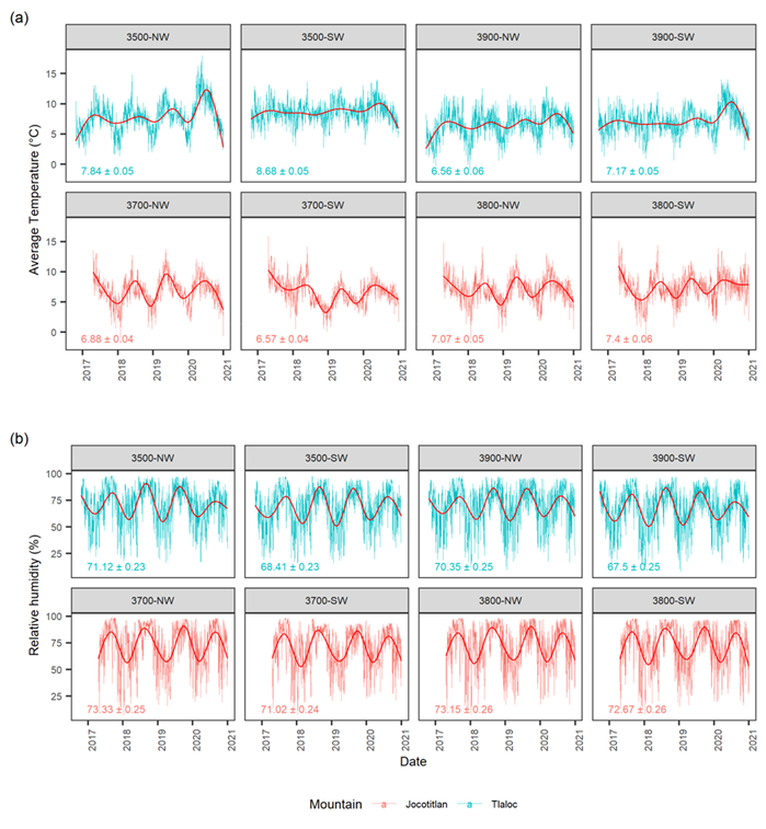
Temperature showed a higher amplitude (maximum-minimum temperature) at high elevations during the winter and spring seasons. For example, site 3900-NW (i.e., combination of elevation and aspect) at TLA showed a temperature variation from -4.8 °C to 35 °C in November, this is a difference of around 40 °C which is remarkably high (Fig. 3a). Lauer (1978) reported similar results in the treeline of Pico de Orizaba (up to 4,000 m asl) where differences were around 44 °C (-7 °C to 37 °C). However, it is important to highlight that compared to air and forest canopy, surface soil variations in temperatures are lower, with biologically suitable temperatures to allow meristem activity in the trunk and the root growth processes (Wieser y Tausz, 2007). Notably, the last recorded year showed the highest average temperature in TLA, nevertheless, due to a low number of years in our database, we cannot asseverate a warming trend (Fig. 3a).
Regarding relative humidity, September was the month with the highest relative humidity (85.1% ± 0.25%) for TLA and JOC (87.4% ± 0.25%) (Fig. 2b). The highest single values were common during the rainy season (June to October) while highly contrasting values for the rest of the year (Fig. 2b). Northern aspects exhibited higher humidity than Southern (p = 0.02) aspects as expected in North hemisphere locations.
Not all sites showed the typical sinewave form on the daily temperature over the year. For example, Southernmost aspects were more prone to show a lower interannual variability than Northern aspects on average temperature (Fig. 3a). Moreover, an unexpected result was the trend found in 3900-NW at TLA for maximum temperature, where high values were almost constant during the studied period. This finding contrasts with the common belief that northern aspects at high elevations present lower maximum temperatures. For relative humidity, all sites reached their maximum during summer and a minimum in winter (Fig. 3b).
The datalogger locations (sites) are defined as a combination of elevation (3500 m, 3700 m, 3800 m, and 3900 m a.s.l.) and aspect (Northwest - NW, and Southwest - SW) within each Mountain. Inset numbers represent the mean value ± standard error. Red lines are splines to highlight daily trends.
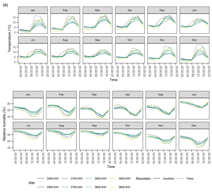
Four-hourly temperature measurements showed a daily cycle characterized by a maximum at 16:00 hours with a decrease during the night and early morning (4:00 am) (Fig. 4a). Conversely, the lowest relative humidity was found at 16:00 hours and the highest during midnight (0:00 am). A reduction in the average relative humidity was found during the dry season (November to May) while high values were more common during the wet season (June to October) (Fig. 4b).
Elevation and aspect as drivers of climatic conditions
Elevation and aspect were relevant factors explaining temperature (p = 0.01 and p = 0.02, respectively) (Table 1). The elevation effect on temperature is a well-known fact establishing that temperature decreases as elevation increases. The theoretical thermal gradient ranged between 0.5°C - 0.6 °C by 100 m in the region (Lauer, 1978). However, the rate of decrease was 0.36 °C by 100 m of elevation at TLA. Thus, the lower thermal gradient found in TLA highlights the requirement for in situ data if the extrapolated data is needed. For example, Astudillo-Sánchez et al. (2019) estimated the mean annual temperature in 4.2 °C at the treeline of TLA (≈ 4000 m a.s.l.) which is lower than our data suggest, even if we corrected for the last 100 m of elevation (6.1 °C). On the other hand, the aspect affects the temperature by an enhanced incoming irradiation and evaporation demand in South aspects (Binkley y Fisher, 2020). Contrary to temperature, elevation was not significant for relative humidity (p = 0.52), but aspect was a significant factor (p = 0.02) (Table 1). In general, northern aspects had higher humidity than southern aspects (p < 0.05), explained by the lower incoming irradiation as described above.
Table 1 Linear mixed model results for temperature and relative humidity.
| Predictors | Temperature | Relative humidity | ||||
| Estimates | S.E. | p-value | Estimates | S.E. | p-value | |
| Intercept | 0.88 | 0.33 | < 0.0001 | 0.95 | 0.32 | 0.03 |
| Mountain | -0.13 | 0.20 | 0.01 | -0.17 | 0.03 | 0.01 |
| Elevation | -0.001 | 0.00 | 0.01 | 0.00 | 0.00 | 0.52 |
| Aspect | 2.82 | 1.20 | 0.02 | -1.11 | 0.77 | 0.02 |
| Time (months) | 0.86 | 0.02 | < 0.0001 | 0.08 | 0.04 | < 0.0001 |
| Time (hours) | 1.32 | 0.01 | <0.0001 | -0.03 | 0.00 | < 0.0001 |
| Elevation x aspect | -0.01 | 0.00 | 0.08 | 0.00 | 0.00 | 0.30 |
| Random effects | ||||||
| 𝜎2 (Residual variance) | 0.28 | 0.71 | ||||
| 𝜏𝜋 (Variance from the random site effect) | 0.03 | 0.01 | ||||
| 𝜏𝛽 (Variance between mountains) | 0.00 | 0.00 | ||||
| Observations | 69 341 | 69 341 | ||||
| Marginal R2 / Conditional R2 | 0.678 / 0.682 | 0.329 / 0.331 | ||||
| Akaike Inf. Criterion (AIC) | 110 446.90 | 94 680.99 | ||||
| Bayesian Inf. Criterion (BIC) | 110 446.90 | 94 937.08 | ||||
Mountain, elevation, aspect, and time (expressed as months and hours) were considered as fixed effects while the datalogger location (site) and repeated measurement were random effects. Both response variables were transformed with the ordered quantile normalization (ORQ) to achieve linear assumptions
The importance of hierarchically organized data in modelling
The hierarchical models accounted for the fact that repeated measurements in time were nested within dataloggers locations (sites) and mountains (Table 1). Furthermore, trought linear mixed models we were able to separate the fixed and random effects on the T and RH. However, a desirable property for random effects is that require at least five levels (e.g. mountains) to achieve a robust estimate of variance (Harrison et al., 2018).
We found that the ORQ was the best normalization transformation for both variables (T and RH). Nevertheless, it is important to highlight that a common issue with transformations is that also affect the relationship between predictors and response, making it difficult the prediction and interpretation of the transformed variables (e.g. logarithm of T). Contrary to other methods, the ORQ transformation is reversible (i.e. one-to-one), thus any analysis performed on transformed data can be interpreted using the original units (Peterson y Cavanaugh, 2020). Once transformed, the addition of an AR2 process (ARIMA2,0,0) to model the temporal autocorrelation coupled with Power variance treatment for residual variance (time-varying across mountains) was better than simple models. Overall, the fixed factors explained ~70% of the T and ~33% for RH (marginal R2). On the other hand, the conditional R2 was slightly higher explained by the combination of fixed factors and accounting for site and time variance (Table 1). Conceptually, random effects resolve the non-independence issue by assuming that the parameters follow a random distribution (usually a normal distribution) across the subjects. Assuming that the intercept in a regression model is the random parameter implies that every site has a different intercept and that these intercepts are assumed to be drawn from a (normal) distribution (Fig. 5a and 5b) (Riha, Güntensperger, Kleinjung y Meyer, 2020). Notably, despite modeling the hierarchy of the data and accounting for their structure, some residual variance remained relatively high, likely due to a strong variability in T over specific days in TLA (Fig. 5c) and the common values close to 100% of RH during the rainy seasons (Fig. 5d).
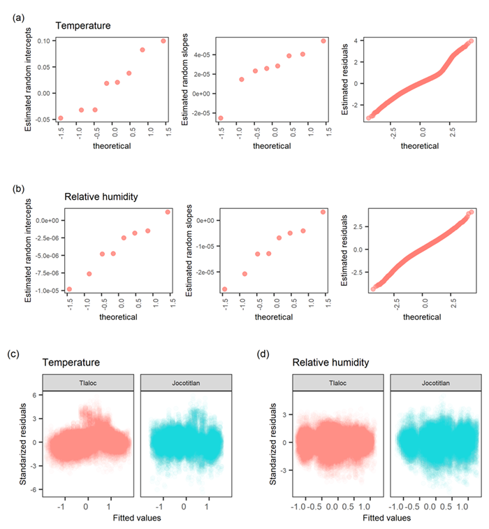
Note that both response variables were transformed with the ordered quantile normalization (ORQ) to achieve linear assumptions.
Figure 5 Probability plots of estimated random intercepts, random slopes, and residuals for (a)Temperature, and (b) Relative humidity; residual plots to tests homogeneity of variance(c) and (d).
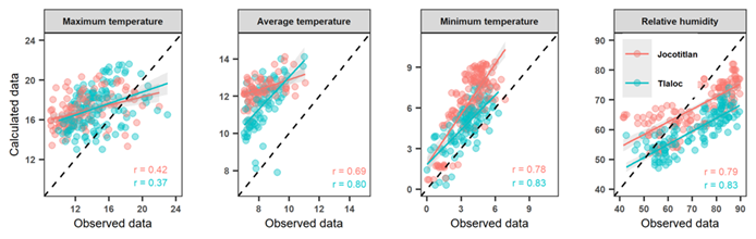
Comparison between downscaled and in situ data Although we found statistically significant correlations between sources and among variables (r = 0.37 to 0.83, p < 0.05, Table 2), some overestimations arise from downscaled data for temperature and underestimations for relative humidity at both mountains (p < 0.001). For example, we found a difference of +3.5 °C for average temperature (7.06 °C vs 10.76 °C, p < 0.001). This difference was more evident for the maximum temperature (+ 4.6 °C, p < 0.001), where low correlations were also found (r = 0.37 and 0.42 for TLA and JOC, respectively) (Fig. 6; Table 2). For minimum temperature, despite that higher correlation (r = 0.83 and 0.78 for TLA and JOC, respectively) were coupled with lower variations (+ 1.18 °C), the differences remained statistically significant (p < 0.001) (Fig. 6). Regarding relative humidity, we found a higher correlation between sources (r = 0.83 and 0.79 for TLA and JOC, respectively) however, calculated data tend to present lower values than observed (≈ 10 %) mainly for the rainy season where differences were about 15%.
Table 2 Linear association between observed and calculated data (ClimateNA derived) by the mountain.
| Variable | Mountain | Pearson correlation | Regression Slope + SE | R2 | R2-adj |
| Maximum temperature | Tláloc | 0.37*** | 0.47 + 0.10 | 0.14 | 0.13 |
| Jocotitlán | 0.42*** | 0.88 + 0.17 | 0.18 | 0.17 | |
| Average temperature | Tláloc | 0.80*** | 0.69 + 0.04 | 0.64 | 0.64 |
| Jocotitlán | 0.69*** | 0.80 + 0.07 | 0.48 | 0.47 | |
| Minimum temperature | Tláloc | 0.83*** | 0.68+ 0.04 | 0.68 | 0.68 |
| Jocotitlán | 0.78*** | 0.50 + 0.03 | 0.62 | 0.61 | |
| Relative humidity | Tláloc | 0.83*** | 1.56 + 0.09 | 0.69 | 0.69 |
| Jocotitlán | 0.79*** | 1.47 + 0.10 | 0.62 | 0.62 |
Average, maximum, and minimum temperatures are expressed in °C while relative humidity is %.
Conclusions
Because of the scarcity of meteorological stations and the strong need for climatic information for alpine forests, the in situ information and the validation with algorithm sources are important. While we confirmed the effect of elevation and aspect on temperature, a lesser-known effect of aspect on relative humidity was revealed. Extreme amplitudes on daily- temperature (around 40 °C) were found at high-elevation sites where less variation is tr aditionally assumed. Although we confirmed statistically significant correlations between derived and instrumental data, the degree of correlation varied among climatic variables. The minimum temperature was the most significantly correlated variable with the large-scale algorithm. Therefore, we propose that whenever possible, downscaled and in situ data should be calibrated for better interpretation of historical and ecological processes in alpine forests.

