


 text new page (beta)
 English (pdf)
 Article in xml format
 Article references
 Send this article by e-mail
 Cited by SciELO
  Similars in
SciELO
Similars in
SciELO 
 Permalink
Introduction
Eucalyptus tereticornis (Smith) is one of the main species used in reforestation programs in Colombia, it participates with 2.13% of the total forest plantation area, estimated at 477 575 ha (World Bank, 2015; Program on Forests [Profor], 2017). In recent years, new plantations have been established with this species, and currently there are more than 10 174 hectares planted mainly on the Colombian Atlantic coast (Profor, 2017). The main aim of these plantations is to supply the regional particle board industry (Obregón & Restrepo, 2007). These forest plantations have been extensively managed, which implies that thinning and pruning are not applied during rotation (Profor, 2017). However, in order to diversify timber production and increase the species profitability, silvicultural regimes that include thinning and pruning must be developed.
Despite its importance, information about the growth and yield of this species is scarce. Hernández (1993) evaluated the effect of different planting densities on E. tereticornis growth, finding that an initial density of 2222 plants per hectare with a spacing of 3.0 m × 1.5 m obtains the highest yield in volume (230 m3 ha-1) at seven years of age. López, Trincado, Barrios, and Nieto (2013) and López, Barrios, and Trincado (2015) fitted regional height-diameter and taper models, respectively, for the species growing on the Atlantic coast.
Reliable information about the dynamics and the development along the rotation of E. tereticornis stands is required to improve management planning (Gonzalez-Benecke et al., 2012). In this process, projection models of tree and stand variables are usually used to predict the growth and volumetric production of the forest (Vanclay, 1994). There are several types of growth and yield models: at the stand level, diameter classes, and individual tree (Guzmán, Morales, Pukkala, & de-Miguel, 2012). Among these, stand models are more widely used in the management of forest plantations due to their relative simplicity and robustness, and the accuracy of their estimates (Burkhart & Tomé, 2012; Santiago-García et al., 2015).
An important component of a stand growth model is the equation that predicts basal area growth (Chikumbo, Mareels, & Turner, 1999; Chikumbo, 2001). This component is relevant for the planning of silvicultural regimes due to its direct relationship with the quadratic mean diameter, volume, and the density of the stand, as a result of the relation between the available space and the volumetric production of trees (Dyer, 1997).
Basal area functions must comply with the following characteristics: a) invariance of the projection (Gadow, Sánchez-Orois, & Álvarez-González, 2007), b) it must consider the assumptions of biological growth, therefore it must have an inflexion point in regards to age (Diéguez-Aranda, Castedo-Dorado, & Álvarez-González, 2005) and a tendency to reach a horizontal asymptote at older ages (Kiviste, Álvarez, Rojo, & Ruiz, 2002; Santiago-García et al., 2015), and c) the formulation must be simple to avoid over-parameterization that leads to multicollinearity (Castedo-Dorado, Diéguez-Aranda, & Álvarez-González, 2007).
Basal area modelling strategies have included the use of equations in algebraic differences (Piennar & Shiver, 1986) and differential equations that estimate the annual or periodic increase (García & Ruiz, 2003). In recent years the interest in models in the form of algebraic differences has increased (Tewari & Gadow, 2005; Gonzalez-Benecke et al., 2012). The formulation of the model as an equation in algebraic differences guarantees compliance with the indicated fundamental properties (Gadow et al., 2007).
The equation that uses algebraic differences is called the projection model, and its use requires information on the initial state variables obtained through a forest inventory in order to project the dependent variable (basal area) to a future state. When no information from a previous forest inventory is available, it is necessary a prediction function of the basal area that allows its value in the initial state to be estimated (Diéguez-Aranda et al., 2005).
Projection and prediction models must produce compatible estimates, therefore, statistical techniques that ensure this characteristic must be used for model fitting (Pienaar, Page, & Rheney, 1999; Tewari, 2007). A commonly used strategy is to estimate the parameters of the projection model and to replace them in the prediction model and subsequently fit the latter model to estimate the non-common parameters (Diéguez-Aranda et al., 2005; Castedo-Dorado et al., 2007). Another strategy is to estimate the projection and prediction parameters of the models simultaneously (Clutter, 1963; Tewari, 2007).
Basal area models are usually developed for unthinned stands (Forss, Gadow, & Saborowski, 1996; Tewari, 2007), however, these models must have the ability to predict the growth of thinned stands. When considering management regimes that include one or more thinnings, the decision-making problem is more complicated, and its analysis requires growth and yield information that incorporates growth responses after thinning (Piennar, 1979).
Objectives
The development of an appropriate basal area growth model for E. tereticornis is necessary to optimize silvicultural management regimes and to achieve diversified production for the species. In this study, nine basal area growth models for unthinned stands were compared and their integration with a thinning response model was examined. The specific objectives were (i) to develop projection and prediction basal area models for unthinned stands of E. tereticornis, (ii) to model the response to thinning through a competition index, and (iii) to evaluate the predictive capacity of the selected models at projecting the growth of unthinned and thinned stands of E. tereticornis in order to be included in a growth and yield projection system for this particular species in Colombia.
Materials and methods
Data
The database used in this study originates from commercial stands of E. tereticornis, located on the Colombian Atlantic coast, between the coordinates 9.3° - 10.8° N and 73.2° - 74.9° W (Fig. 1). This area is characterized by flat topographies, with slopes that do not exceed 5% and with average altitudes of 50 meters above sea level. The average temperature is 28 °C and the average annual rainfall is 1350 mm year-1. The soils that predominate are plains with an alluvial, fluviomarine, and wind origin, with sandy-clay textures, pH between 4.1 and 5.5, little organic matter and nutrient content (Barrios, López, & Nieto, 2011).
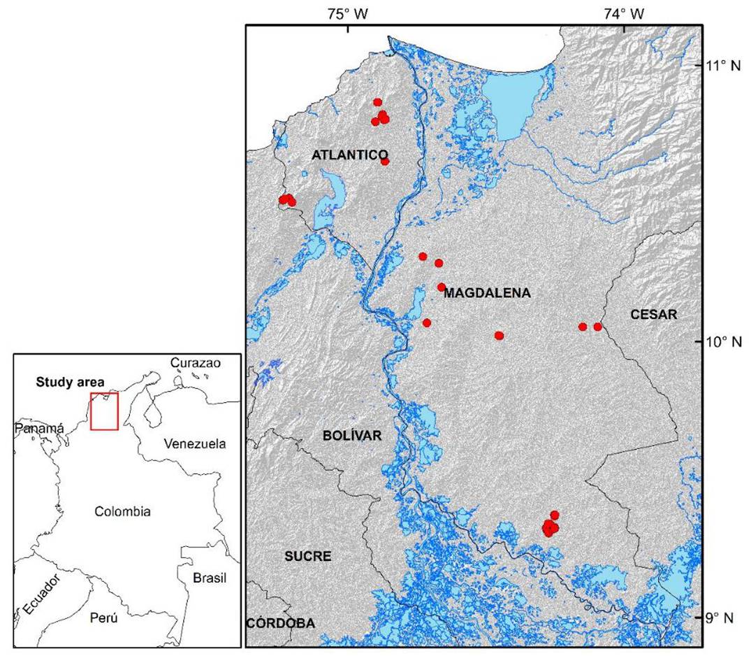
FIGURE 1 Geographic location of the study area. Location of permanent and thinning plots are indicated as red dots.
For this study, 97 permanent unthinned plots with at least two consecutive measurements were used. A total of 86 circular permanent plots between 500 m2 and 800 were installed and measured during the period 2008-2013, with 2 to 5 measurements. Additionally, 11 rectangular permanent plots with a surface of 1000 m2 that were installed and measured during the period 1992-1995 (3 measurements) were also available for the study (Table 1).
TABLE 1 Descriptive statistics of the data used for model development.
| Variable | Permanent plots (97 plots) | Thinning plots (72 plots) | ||||||
| Mean | Minimum | Maximum | SD | Mean | Minimum | Maximum | SD | |
| t | 6.1 | 1.2 | 12.6 | 2.6 | 6.9 | 5.0 | 9.0 | 1.1 |
| H | 18.8 | 6.2 | 30.6 | 4.6 | 18.5 | 11.6 | 24.0 | 2.8 |
| N | 1008 | 180.0 | 3792.0 | 407.4 | 873.6 | 414.0 | 1656.1 | 291.2 |
| G | 10.5 | 0.9 | 20.1 | 4.2 | 10.1 | 2.2 | 18.3 | 3.1 |
| S | 25.1 | 18.1 | 31.6 | 2.7 | 22.7 | 17.4 | 26.7 | 2.0 |
t: age (years); H: dominant height (m); N: number of trees (ha-1); G: basal area (m2 ha-1); S: site index (m) at base age of 10 years; SD: standard deviation.
To incorporate the thinning response on the basal area growth, data from six thinning trials installed in stands of 5, 6 and 7 years-old were used, with thinning intensities ranging from 10% to 40% of basal area removed. Thinnings were selective from below; meaning that the trees suppressed, dead or malformed had the highest priority to be thinned, when trying to leave desirable trees evenly spaced within the stand. These trials were measured during 2009-2011 and have 2 measurements after thinning (Barrios et al., 2011). After debugging the information, 72 plots were selected to fit a competition index model (Table 1).
The same measurement protocol was used for both permanent plots and thinning trials. The following variables were recorded for each selected tree within each plot: diameter (d) measured at 1.3 m above the ground with diametric tape and the total height (h) was measured with a vertex laser hypsometer (Haglög) to a sample of trees. The missing heights for each plot were predicted by fitting the local height-diameter model proposed by Flewelling and Jong (1994) in each re-measurement. The dominant height (H) corresponds to the average height of the 100 trees ha-1 with the largest diameter. The site index (S) was calculated for each plot by using the fitted model of López, Barrios, Trincado, and Nieto (2011),
where:
S: site index
H: dominant height at age t
Modelling of basal area for unthinned stands
For this study, nine previously reported models were selected for evaluation and comparison (Table 2). The main difference between the models is the number of parameters to be estimated and the stand-level variables included in their structure. As a response variable, a logarithmic transformation was preferred, since it allows the heterogeneity of the variances to be controlled, approaching normality (Gonzalez-Benecke et al., 2012).
Modelling the basal area for thinned stands
The response to thinning on basal area growth was modelled following the methodology reported by Pienaar (1995). A competition index (CI), was defined as,
where:
GU: basal area in the unthinned plot
GT: basal area in the thinned plot
In equation 2 it can be observed that when GT is equal to GU, the CI is zero. When GT is less than GU (case of operational thinning), the CI is greater than zero, but will tend to approach zero as the stand grows. The CI (Eq. 2) was calculated for each measurement, dividing the basal area of each thinned plot by the basal area of the closer unthinned control plot. Both plots had approximately the same density and site quality at the time of thinning. An equation to predict the expected CI trend was fitted to these data according to the age and the dominant height,
where:
CIi and CIj: competition index
Hi and Hj: dominant height at age ti and tj (j > i), respectively
α1 and α2: parameters to be estimated
εk: error, with εk ~ N (0, σ2)
To calculate the basal area of thinned stands, the selected basal area model for unthinned stands (Table 2) is combined with equation 3, using the projected CIj,
where:
GTj: basal area of the thinned stand at age j
GUj: basal area of the unthinned stand at age j
TABLE 2 Basal area projection and prediction models for unthinned stands.
| Model | Author | Projection model | Prediction model |
| 1 | Bennett (1970) | lnG j =lnG i ⋅ (t i/t j )+β1 ⋅ (1- ti/t j )+εk | lnG i = (β 0 +β1 ⋅ t i ) /t i +εk |
| 2 | Borders and Bailey (1986) | lnG j =lnG i +β1 ⋅ (lnH j -lnH i )+εk | lnG i =β 0 +β1 ⋅ lnH i +εk |
| 3 | Clutter (1963) | lnG j =lnG i ⋅ (t i/t j )+β1 ⋅ (1- t i/ t j )+β 2 ⋅ (1- t i/t j )⋅S+εk | lnG i = (β 0 +β1 ⋅ t i +β 2 ⋅ t i ⋅S )/ t i +εk |
| 4 | Forss (1994) | lnG j =lnG i +β1 ⋅ (1/ t j -1/t i )+β2 ⋅ (lnHj -lnHi )+εk | lnG i =β 0 +β1 ⋅ (1/t i ) +β 2 ⋅ lnH i +εk |
| 5 | Gurjanov et al. (2000) | lnG j =lnG i ⋅ (t i/t j )+β1 ⋅ (1- ti/t j ) +β2 ⋅ (lnN j -(ti /t j )⋅ lnNi )+εk | lnG i = (β 0 +β1 ⋅ t i +β 2 ⋅ t i ⋅ lnN i )/t i +εk |
| 6 | Hui and Gadow (1993) | lnG j =lnGi + (1-β1 ⋅ Hβ j 2 )⋅ lnN j +(β1 ⋅ Hβ i 2 -1) ⋅ lnNi +β3 ⋅ (lnH j -lnHi )+εk | lnG i =β 0 + (1-β1 ⋅ Hβ i 2)⋅ lnN i +β 3 ⋅ lnH i +εk |
| 7 | Forss et al. (1996) | lnG j =lnG i +β1 ⋅ (1 t/j -1/ti )+β2 ⋅ (lnN j -lnNi ) +β3 ⋅ (lnH j -lnHi )+εk | lnG i =β 0 +β1 ⋅ (1/t i ) +β 2 ⋅ lnN i +β 3 ⋅ lnH i +εk |
| 8 | Souter (1986) | lnG j =lnG i ⋅ (t i/t j )+β1 ⋅ (1- ti/t j )+β 2 ⋅ (1- t i/t j )⋅S+β3 ⋅ (lnN j -(ti /t j )⋅ lnNi )+εk | lnG i = (β 0 +β1 ⋅ t i +β 2 ⋅ t i ⋅ S+β 3 ⋅ t i ⋅ lnN i )/t i +εk |
| 9 | Pienaar and Shiver (1986) | lnG j =lnGi +β1 ⋅ (1 t/j -1/ti )+β2 ⋅ (lnN j -lnNi )+β3 ⋅ (lnH j -lnHi ) +β4 ⋅ (lnN j/t j - lnNi/ti ) +β5 ⋅ (lnHj/tj - lnHi ti )+εk | lnG i =β 0 +β1 ⋅ (1/ t i ) +β 2 ⋅ lnN i +β 3 ⋅ lnHi/+β4 ⋅ (lnNi/ti ) +β5 ⋅ (lnHi /ti ) +εk |
Gi and Gj is the basal area per hectare, Hi and Hj is the dominant height, Ni and Nj is the number of trees per hectare at age ti and tj (j > i), respectively; S is the site index, βl are the parameters to be estimated (l = 0, 1, 2… p), ln is the natural logarithm and εk is the random error.
Estimation of parameters and validation of models
To fit the projection and prediction basal area models, the parameters of both equations were estimated simultaneously. This strategy minimizes the sum of squares of the error of the entire system, optimizing the fitting of both functions (Tewari, 2007). The parameter estimation of the basal area and competition index models was performed using the MODEL procedure contained in the statistical software, Statistical Analysis System (SAS Institute Inc., 2009). During the fitting process the minimization algorithm of the sum of squares of the error used was Gauss-Newton. To guarantee convergence in a global optimum, different initial parameters obtained from previous studies were used. The goodness of fit of the models was evaluated using the standard error of the estimate,
And the adjusted coefficient of determination, defined as,
where:
yi: observed dependent variable
ŷi: predicted dependent variable
ȳ: observed dependent variable average
n: total number of observations
p: number of model parameters.
Due to the small number of plots, a cross-validation process (k-fold cross-validation) was used to evaluate the models (Refaeilzadeh, Tang, & Liu, 2009). This process consisted in estimating the parameters of each model over 10 opportunities. At each opportunity, a group of plots was randomly left out (~ 10 and ~ 7 plots for basal area and competition index models, respectively) and the residuals of their observations were calculated. This procedure allowed model validation with a different sample from that used in the fitting process.
To correct the bias from the logarithmic transformation used in the basal area models, we used the methodology proposed by Baskerville (1972) and described by Lee (1982). Measures of goodness of prediction (bias and error) were calculated with the residuals generated in the cross-validation process. As a measure of bias, the mean error was used
The root of the mean square error was used as a measure of error,
yi: observed value
ŷi: predicted value
n: number of observations
The models were ranked according to their value of the goodness of prediction statistics, then the models were ranked by adding the values obtained for each statistic for the projection and prediction models. The residuals generated by each model were analysed graphically to evaluate normality and homogeneity of variances. The best model was the one that presented the best prediction statistics (better ranking), its residuals showed no anomalous tendencies and its evolution curves according to age presented a biologically logical behaviour. The predictive capacity of the equation system, formed by the basal area model selected for unthinned stands and the competition index, was evaluated during the prediction of the basal area after thinning using the same statistics (ME and RMSE).
Practical application
To exemplify the use of the system of basal area projection and prediction equations, and the developed competition index model, these were used to predict the growth of two hypothetical E. tereticornis stands with the same initial planting density (1333 trees ha-1) and a survival rate of 90% after the first year. The simulated stands had site indexes: 20 and 30 m. The mortality model proposed by López et al. (2011) was used to quantify the reduction in density until the first thinning,
Ni and Nj: density (trees ha-1) at age ti and tj (j> i), respectively.
Stands were simulated with no thinning and with thinning (two thinnings, removing 33% of basal area at the age of 6 and 9 years). The simulation length was defined as 12 years, similar to the species rotation projection (Madeflex, 2010).
Results
Model fitting
Table 3 shows the estimated parameters, standard errors, the probability value, and the goodness of fit measurements for the projection and prediction models fitted by the simultaneous fitting procedure. All the models evaluated presented highly significant parameters (P < 0.01), except model 5, where parameter β1 was not significant (P > 0.05). We observed that the stand-level variables incorporated as independent variables in each model analysed had a significant effect on the basal area development of the evaluated stands.
TABLE 3 Parameter estimates and goodness of fit for basal area projection and prediction models, and for the competition index.
| Model | Parameter | Estimate | Standard error | P-value | Projection | Prediction | ||
| Syx | R 2 adj | Syx | R 2 adj | |||||
| 1 | β0 | -3.459490 | 0.1154 | <0.0001 | 0.122 | 0.913 | 0.289 | 0.689 |
| β1 | 2.968428 | 0.0271 | <0.0001 | |||||
| 2 | β0 | -2.324760 | 0.1092 | <0.0001 | 0.128 | 0.904 | 0.250 | 0.767 |
| β1 | 1.594247 | 0.0383 | <0.0001 | |||||
| β0 | -3.645780 | 0.1069 | <0.0001 | 0.123 | 0.912 | 0.254 | 0.760 | |
| 3 | β1 | 1.709039 | 0.1415 | <0.0001 | ||||
| β2 | 0.051926 | 0.0057 | <0.0001 | |||||
| β0 | -0.552390 | 0.2169 | 0.0115 | 0.114 | 0.924 | 0.236 | 0.793 | |
| 4 | β1 | -1.346670 | 0.1452 | <0.0001 | ||||
| β2 | 1.076249 | 0.0663 | <0.0001 | |||||
| β0 | -3.556830 | 0.1109 | <0.0001 | 0.123 | 0.913 | 0.268 | 0.732 | |
| 5 | β1 | 0.641283 | 0.3322 | 0.0547 | ||||
| β2 | 0.340440 | 0.0485 | <0.0001 | |||||
| β0 | -11.622700 | 0.3722 | <0.0001 | 0.117 | 0.920 | 0.203 | 0.847 | |
| 6 | β1 | 0.112300 | 0.0176 | <0.0001 | ||||
| β2 | 0.580083 | 0.0393 | <0.0001 | |||||
| β3 | 3.870445 | 0.1561 | <0.0001 | |||||
| β0 | -3.725710 | 0.3686 | <0.0001 | 0.115 | 0.923 | 0.198 | 0.854 | |
| 7 | β1 | -1.261990 | 0.1356 | <0.0001 | ||||
| β2 | 0.415648 | 0.0404 | <0.0001 | |||||
| β3 | 1.177248 | 0.0624 | <0.0001 | |||||
| β0 | -3.763600 | 0.0993 | <0.0001 | 0.124 | 0.910 | 0.225 | 0.812 | |
| 8 | β1 | -0.914730 | 0.3246 | 0.0052 | ||||
| β2 | 0.055064 | 0.0051 | <0.0001 | |||||
| β3 | 0.372700 | 0.0425 | <0.0001 | |||||
| β0 | -2.352740 | 0.5463 | <0.0001 | 0.116 | 0.922 | 0.194 | 0.860 | |
| β1 | -8.281140 | 2.0684 | <0.0001 | |||||
| 9 | β2 | 0.249251 | 0.0686 | 0.0003 | ||||
| β3 | 1.076051 | 0.0651 | <0.0001 | |||||
| β4 | 0.773393 | 0.2699 | 0.0045 | |||||
| β5 | 0.715563 | 0.1958 | 0.0003 | |||||
| ICj | α1 | -0.632905 | 0.1703 | 0.0003 | 0.031 | 0.865 | - | - |
| α2 | -1.073414 | 0.2629 | <0.0001 | |||||
For the basal area projection models, R2 adj and Syx varied between 0.90 - 0.92 and between 0.114 - 0.128, respectively. The basal area projection models that presented the best goodness of fit were 4, 7, 9 and 6 (Table 3). These last three models also presented better goodness of fit considering the prediction models (Table 3). For the basal area prediction models the R2 adj and Syx varied between 0.69 - 0.86 and between 0.194 - 0.289, respectively.
Model validation
The ME varied between -0.519 m2 ha-1 and 0.281 m2 ha-1 and the RMSE was between 1.080 m2 ha-1 - 1.343 m2 ha-1 for the projection models. Within the evaluated group of basal area projection models, models 1, 3, 9, 6, 5 and 7 stood out with the lowest average errors. Regarding the prediction models, the ME varied between 0.004 m2 ha-1 - 0.086 m2 ha-1 and the RMSE between 1.671 m2 ha-1 - 2.206 m2 ha-1. Of the evaluated basal area prediction models, models 9, 7, 8 and 6 stood out with the lowest average errors (Table 4). The models with the best performance in both the projection and the prediction basal area were models 9 (sum of ranks = 13), 6 (sum of ranks = 15) and 7 (sum of ranks = 17).
TABLE 4 Measures of goodness of prediction and sum of ranks for basal area (m2 ha-1) projection and prediction models for unthinned stands.
| Model | Projection | Prediction | Sum of ranks | ||
| ME | RMSE | ME | RMSE | ||
| 1 | 0.250 (4) | 1.080 (1) | 0.035 (7) | 2.206 (9) | 21 |
| 2 | -0.519 (9) | 1.343 (9) | 0.004 (1) | 2.073 (8) | 27 |
| 3 | 0.138 (1) | 1.090 (2) | 0.086 (9) | 2.045 (7) | 19 |
| 4 | -0.383 (8) | 1.126 (7) | 0.030 (6) | 1.941 (5) | 26 |
| 5 | 0.281 (6) | 1.122 (5) | 0.018 (3) | 1.958 (6) | 20 |
| 6 | -0.153 (2) | 1.114 (4) | 0.028 (5) | 1.779 (4) | 15 |
| 7 | -0.342 (7) | 1.123 (6) | 0.011 (2) | 1.691 (2) | 17 |
| 8 | 0.165 (3) | 1.133 (8) | 0.076 (8) | 1.778 (3) | 22 |
| 9 | -0.253 (5) | 1.105 (3) | 0.026 (4) | 1.671 (1) | 13 |
Note: values in brackets indicate the position occupied by the model for each statistic. The models with the lowest sum of ranks are underlined.
These models were evaluated graphically to assess their biological behaviour and their predictive capacity (Fig. 2). When analysing the basal area curves of evolution of these models, we observed that model 6 presents a deficient behaviour in its asymptote, which causes it to cross growth paths for some of the evaluated plots (Fig. 2a). On the contrary, models 7 and 9 did not present this problem. In general, these two models adequately describe the basal area growth trajectories of the evaluated plots. However, model 7 shows better biological behaviour, maintaining an appropriate asymptote for the basal area growth of the species (Fig. 2 b, 2c). This model presents considerable superiority compared to the other models evaluated and its predictions remain stable over a wide range of input values. The projection model residuals (model 7) are randomly distributed over the range of predicted values and no particular systematic trend was observed (Fig. 3 a, 3b). Similar behaviour was observed in the prediction model residuals; however, they tend to increase as the basal area predicted for the stand increases (Fig. 3 c, 3d). This means that the prediction model presents a greater error in the prediction of basal area in dense stands.
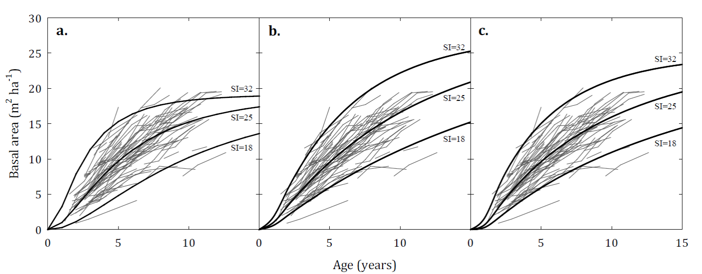
FIGURE 2 Basal area development curves generated from the models of (a) model 6, (b) model 7 and (c) model 9 for site indexes 18 m, 25 m and 32 m and a stand density of 1000 trees ha-1 superimposed on the observed basal growth trajectories.
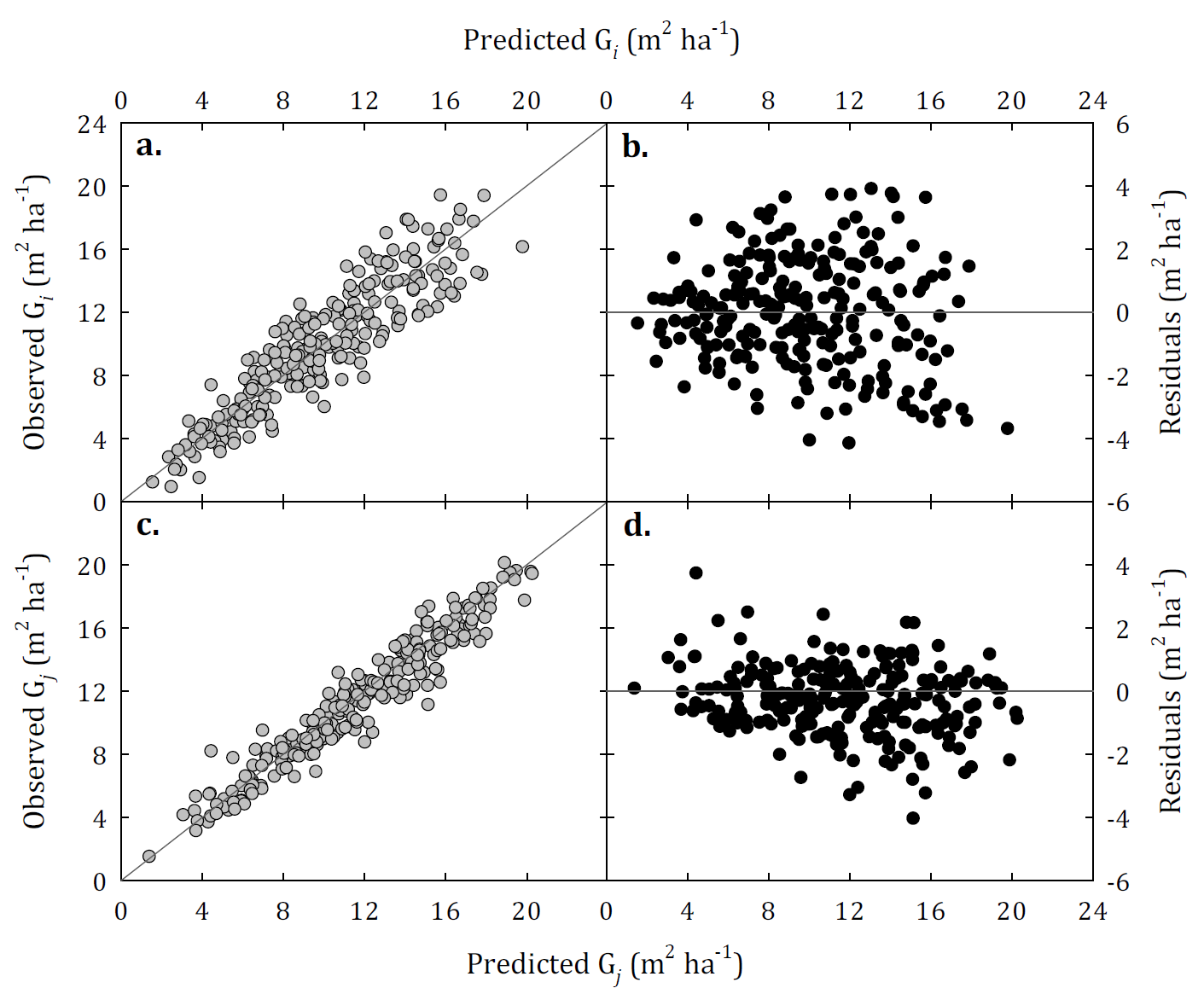
FIGURE 3 Observed and predicted basal area and residual dispersion for unthinned stands using the model 7 (Forss et al., 1996) prediction (a, b) and projection (c, d) models, respectively.
Thinning response model
The model that projects the competition index after thinning was dependent on age and dominant height of the stand (Eq. 3). This model showed a satisfactory fit with an R2 adj of 0.866 and a Syx of 0.031% (Table 3). A scatter plot between the observed and predicted values for CIj indicates a high degree of association between these values and the absence of bias in the predictions (Fig. 4a), likewise, the residuals are distributed randomly along the range of predicted values (Fig. 4b). The observed and predicted values for the basal area (Fig. 4c) after thinning joining the model 7 and the competition index, presents an adequate association, with errors distributed within the range of predicted values (Fig. 4d). The system of equations presented a slight tendency to overestimate with a ME of - 0.14 m2 ha-1 and a RMSE of 0.696 m2 ha-1.
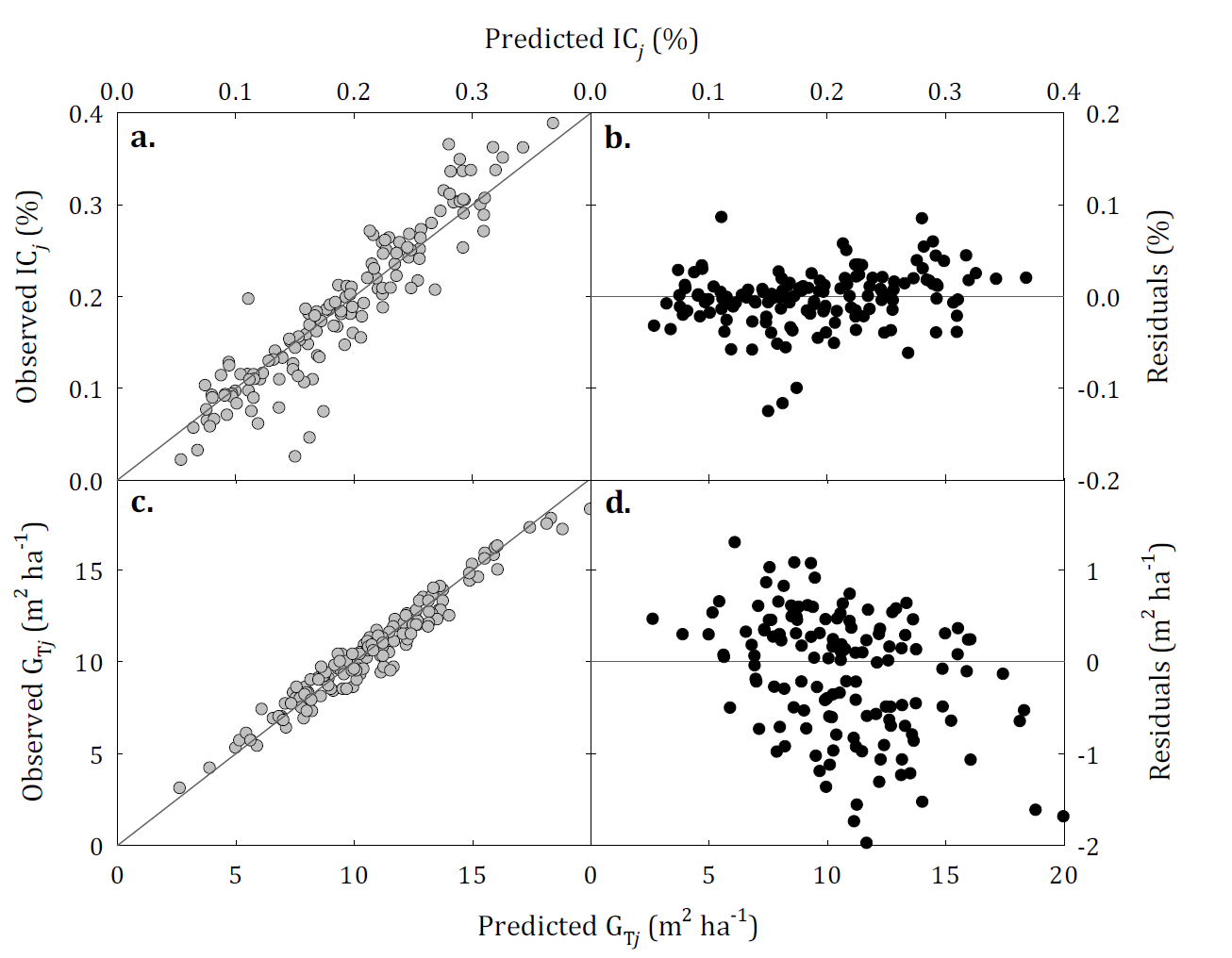
FIGURE 4 Observed and predicted competition index (a) and basal area after thinning (c) and residual dispersion (b, d) for thinned stands. After the thinning, basal area is predicted joining the model 7 (Forss et al., 1996) model and the competition index.
Practical application
A practical application of the models developed to predict the growth of hypothetical E. tereticornis stands planted with 1333 trees ha-1 at site indexes of 20 m and 30 m is presented in the figure 5. As shown, the system developed is quite sensitive to variations in site quality (site index). The unthinned stands growing at site indexes of 20 m and 30 m reached a basal area of 14.03 m2 ha-1 and 21.48 m2 ha-1, respectively, at the age of 12 years (Fig. 5a). The exponential coefficient of the model represents an average annual CI decline rate as the stand ages after thinning of 4.3% and 3.7%, for site indexes of 20 m and 30 m, respectively.
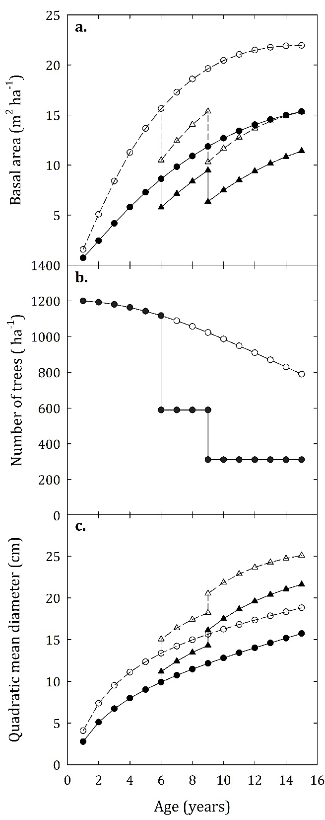
FIGURE 5 Evolution of the basal area, number of trees and quadratic mean diameter for unthinned (circles) and thinned (triangles) hypothetical stands of E. tereticornis growing at two site indexes: 20 m (continuous line) and 30 m (dashed line). The reduction in number of trees (ha-1), calculated with equations 9 and 10, is not affected by site quality, therefore, both evaluated stands present the same evolution in terms of stand density.
Because the thinnings are selective by size, the percentage of trees removed in the thinning is not equal to the percentage of basal area extracted. In such cases the number of trees to be extracted can be calculated using the following model fitted from the thinning trial data (R2 adj = 0.97),
where:
NA and GA: number of trees and basal area at the time of thinning
Next and Gext: number of trees and basal area extracted during thinning.
When the scenario of two thinnings is applied to the stands, the total basal area produced (adding the extracted basal area from thinning to the basal area at the age of 12 years) was 15.4 m2 ha-1 and 23.9 m2 ha-1, equivalent to an increase of 10% and 11% compared with the unthinned stand, for site index 20 m and 30 m, respectively (Fig. 5a). As seen in figure 5b, 528 and 278 trees are removed in the first and second thinning, respectively (Fig. 5b). Additionally, as a result of the elimination of trees that were smaller in diameter during the thinning, the stands increased their quadratic mean diameter by 40% (5.6 cm) and 36% (6.3 cm) at the age of 12 years compared to unthinned stands, for the site indexes 20 m and 30 m (Fig. 5c).
Discussion
In the study, nine projection and prediction basal area models were compared according to their goodness of fit and predictive capacity. The best evaluated models were those that included age, density, and dominant height of the stand as independent variables. The use of an equation to model the response to thinning was a flexible and practical method to evaluate the effect of thinning on basal area growth.
In general, the projection model was more accurate compared to the basal area prediction model. Similar results were reported by Diéguez-Aranda et al. (2005) and Castedo-Dorado et al. (2007). Consequently, the final error when using the basal area function system is conditioned to the prediction model, which can contribute a lot of error in the final result of a simulation (Diéguez-Aranda et al., 2005). Therefore, the values to initiate the projection model should ideally come from a forest inventory and the prediction model should only be used when there is no previous information available (Castedo-Dorado et al., 2007).
The Piennar and Shiver (1986) model produced the lowest average error in the validation stage for the prediction model and the third lowest average error for the basal area projection model. However, this model had excessive parameterization that lead to multicollinearity problems that can affect the significance of certain parameters (Diéguez-Aranda et al., 2005). The model by Forss et al. (1996), which is a modification of the Piennar and Shiver (1986) model, has two parameters less, which is an advantage in terms of parsimony, reducing the risks of multicollinearity. A graphical analysis showed that this model describes the growth trajectories in the basal area (Fig. 2) better than the Piennar and Shiver (1986) model. Therefore, the model by Forss et al. (1996) is selected for the projection and prediction of basal area for unthinned stands of E. tereticornis in Colombia.
Similar to the results obtained in this study, Tewari (2007) found that the models of Forss et al. (1996) and Pienaar and Shiver (1986) reliably described basal area growth trajectories of unthinned Eucalyptus camaldulensis plantations in India. These equations were also applied successfully for the prediction of basal area in red spruce (Gurjanov, Orios, & Schröder, 2000). Maestri, Sanquetta, and Arce (2003) selected the model by Forss et al. (1996) to model basal area growth of Eucalyptus grandis in Brazil. Both models include age, density, and dominant height of the stand as independent variables. These variables have previously been identified as the main sources of variation in basal area models for the Eucalyptus genus (Amaro, Tomé, & Themido, 1997; Dias, Garcia, Chagas, Couto, & Ferreira, 2005; Silva, Chagas, Garcia, Lopes, & Lopes, 2006; Tewari, 2007).
Amaro et al. (1997) developed basal area models for Eucalyptus globulus in Portugal, using the Korf model as a basis, and the site index and stand density as covariates. Dias et al. (2005) fitted the basal area model proposed by Clutter (1963) for hybrid plantations of E. grandis × Eucalyptus urophylla in Brazil, which is dependent only on the initial and projection age. Similarly, Silva et al. (2006) fitted a basal area growth model which included age and site index for plantations of E. urophylla and Eucalyptus cloeziana in Brazil.
The projection of the basal area of thinned stands, using an approach proposed by Piennar (1995), which uses a CI and the basal area of a unthinned counterpart, proved to be a flexible and practical method to include the effect of thinning on growth in the basal area of E. tereticornis. The original Piennar (1995) model only included the age of the stand as an independent variable to model the decline of the CI. Gonzalez-Benecke et al. (2012) also modelled the change in CI depending on stand age. In the present study, the model that predicts the decrease in CI as the stand ages after thinning requires age and dominant height of the stand to be considered as independent variables. Therefore, the developed model has a wider range of applications when considering the effect of site quality in addition to age.
Considering that information from the thinning trials with intensities lower than 50% were used for model fitting, it is recommended that the simulation of thinning scheme scenarios must be conditioned to simulate thinning with these characteristics. In these cases, basal area of a unthinned stand should be projected until the final simulation age, the age and intensity of the thinning should be defined, and the initial CI should be calculated. Basal area after thinning is then calculated for the stand. From this stand condition, the future CI and basal area for the thinned stand is also calculated (Piennar, 1995).
Practical application of the developed models showed that E. tereticornis reaches basal areas of 14.03 m2 ha-1 - 21.48 m2 ha-1 at an age of 12 years and 1333 trees ha-1 for site indexes 20 - 30 m, respectively in unthinned stands. Previous studies for Eucalyptus globulus in Argentina report 32.6 m2 ha-1 of basal area at the age of 10 years for a density of 1095 trees ha-1 (Ferrere, López, Boca, Galetti, Esparrach, & Pathauer, 2005). The best thinning regime for E. tereticornis is beyond the scope of the present study and will vary according to the aim of the plantation. However, the use of the developed models showed that stands with site indexes of 20 m and 30 m, thinned with an intensity of 33% at the age of 6 and 9 years, allowed increased basal area production between 10% and 11% and increased quadratic mean diameter between 36% and 40% compared to unthinned stands. Similar results were reported by Ferraz, Mola-Yudego, González-Olabarria, and Scolforo (2018) for Eucalyptus plantations in Brazil, where thinning regimes applied after 5.5 years, leaving a large number of residual trees, presented the highest production values in basal area.
This study allowed to evaluate and select models to predict basal area growth and simulate the thinning response for E. tereticornis stands grown on the Colombian Atlantic coast. The system of equations developed proved to be consistent, however, caution should be observed when applying these models due to the low number of permanent plots used for their development. More research is required to include a wider range of site conditions, management regimes and genetics to improve the capabilities of the models developed.
Conclusions
The present study identified the Forss et al. (1996) model as the most appropriate for the prediction of basal area of E. tereticornis in unthinned plantations on the Colombian Atlantic coast. The developed equations system includes a function for the projection of basal area based on an initial stand basal area, age, density, and dominant height at the beginning and at the end of the projection period and a basal area prediction model, which acts as an auxiliary model to determine the basal area for any combination of stand age, density, and dominant height. The simultaneous fitting procedure that was used ensures compatibility between the predictions of both models, because the projection and prediction models share parameters in their formulation. The competition index model developed to incorporate the thinning effect on basal area development of E. tereticornis proved to be flexible and practical when determining the basal area of thinned stands. The fitted model predicts the decreased competition index after thinning based on age and the dominant height of the stand.

