


 nueva página del texto (beta)
 Inglés (pdf)
 Artículo en XML
 Referencias del artículo
 Enviar artículo por email
 Citado por SciELO
  Similares en
SciELO
Similares en
SciELO 
 Permalink
Introduction
The structural characterization of a mangrove forest is a mandatory step in the evaluation of mangrove areas (Pool, Snedaker, & Lugo 1977; Cintrón & Schaeffer-Novelli, 1983; Timm & Araújo, 2018). Forest structure-a descriptive measure of important attributes of the vegetation-provides a snapshot of mangrove forest development and health (Pool et al., 1977; Cintrón & Schaeffer-Novelli, 1983; Datta & Deb, 2017). The calculation of structure also permits the delineation of mangrove areas based on similar attributes and allows for baseline assessments and intersite forest comparisons (Cintrón & Schaeffer-Novelli, 1985; Timm & Araújo, 2018). Although the methods used in the calculation of mangrove forest structure were developed for general forestry use, in the 1970s, mangrove ecologists began the process of choosing and standardizing a set of structural attributes that would allow for the characterization of mangrove stands in a wide array of geographical areas (Pool et al., 1977; Martínez, Cintrón & Encarnación, 1979; Schaeffer-Novelli, Cintrón, & Adaime, 1980; Jiménez, 1981). The protocol was formalized in a classic paper by Cintrón and Schaeffer-Novelli (1984), which provided for a standardized set of methods and techniques to study mangrove structure. Since then, the methodology has been applied by many researchers around the world (Araújo & Polanía, 1985; Cintrón & Schaeffer-Novelli, 1985; Day, Conner, Day, Ley-Lou, & Navarra, 1987; Finn, 1996; Fromard et al., 1998; Lovelock, Feller, McKee, & Thompson, 2005; Timm & Araújo, 2018) and has been used in country-wide assessments and management of mangrove areas and resources (Instituto de Recursos Naturales y del Ambiente [Irena], 1986; Jiménez, 1994; Sánchez-Páez & Alvarez-León, 1997; Araújo, 2006; Arden & Price/University of Miami, 2008).
Typically, mangrove forest structure has been investigated using either fixed-area plot or plotless sampling. Fixed-area plots are a fixed area that is selected within which all trees are measured. Plotless sampling does not rely on a specific area, but on several point samples chosen (for a description of the sampling techniques seeCintrón and Schaeffer Novelli, 1984). Given the intrinsic difficulty of sampling mangrove stands, the methods chosen to study structure were designed to be fairly simple, time and cost effective, and universally applicable (Cintrón & Schaeffer-Novelli, 1984). These sampling techniques deliver an array of structural attributes (primary metrics) out of which number of species, tree diameter and height, and stand density are the most common and appear in most publications detailing the structural characteristics of mangrove forests. These primary metrics are then used to calculate a set of secondary metrics (e.g., basal area and relative values of density, dominance, and frequency) that are computed to species level for a detailed description of structural attributes as they apply to each species found. Additionally, structural indices can be calculated using structural data, most common of which are the complexity index (Holdridge, 1967) and mean stand diameter (Cintrón & Schaeffer-Novelli, 1984). For the most part, the indices and formulae used in structure calculations are not particularly complex, but they require a multi-step approach in which the data set that has been collected in the field is parsed, sorted by species, and cross-referenced in a series of steps that are fairly easy to mishandle, and susceptible to mistakes.
To facilitate the calculation of mangrove forest structural parameters, a package for the R environment (mangroveStructure) was developed to automate the process and programmatically provide for the most-commonly applied indices used in structural evaluations, without the uncertainty for miscalculation, and with the convenience and speed that automated computation provides.
Methods
The package mangroveStructure was written for R, a free software and programmatic environment for statistics and graphics. The program runs on the most popular computer platforms including Windows, MacOS, and UNIX. Since its inception in the early 1990s, R has been used by programmers, scientists, and code developers to produce user-created “packages” that ensure reproducible code and results (Wickham, 2015). These packages run specialized statistical functions, produce maps and graphics, and allow researchers to import and export from large data sets in the public domain, among other uses. To date, many thousands of these packages have been developed in virtually all scientific fields and disciplines (Smith, 2017).
Development of the mangroveStructure package followed coding and compilation guidelines outlined by Wickham (2015). Functions and metadata files for mangroveStructure were created and deposited on GitHub on 25 April, 2017, after which a substantial testing period was started. Students at the Rosenstiel School of Marine & Atmospheric Science, University of Miami, were assigned projects as part of a graduate class that necessitated the use of the mangroveStructure package, and their experiences were used to troubleshoot and debug the package code for improved user experience and accuracy.
A summary of required input variables is provided below for both plot and plotless sampling techniques. Input names appear as the default names written for the package, but these argument names can be modified to match any name specified by the user in his/her data set:
Plot data
plotnumber: Sequential integer values starting with 1. If plots are character strings or are nonsequential values, they must be converted.
tree: Unique value to identify every individual tree in the dataset (recommended but not required for analysis). In our example, trees have been sequentially numbered starting with 1.
species: Species or species code of plants found within the plot written as any meaningful string value (e.g., Rhizophora mangle, R. mangle, Rm, red mangrove, etc.). This name will be used by the package to identify each species in all output tables and graphics. The name for each species must be consistent (i.e., same spelling, capitalization, spacing, etc.), or the package will not recognize them as the same species (e.g., R. mangle and R. Mangle will be treated as two distinct species).
dbh: Tree diameter at breast height (DBH) in centimeters.
height: Tree height in meters. This is an optional input that is not necessary for basic analysis, but when present will produce additional height-related outputs related to tree and canopy heights.
plot.width: Numerical argument to specify the width of the plot. Default is 10 m but this number can be modified as needed.
plot.length: Numerical argument to specify the length of the plot. Default is 10 m, but this number can be modified as needed.
Plotless data
samplingpoint: Sequential integer value of each sampling point along the transect, starting with 1.
quarternumber: Sequential integer values from 1 to 4 that denote the four quarters that are established on each sampling point along the transect.
dist: Distance (in meters) from the center of the sampling point to the midpoint of the nearest tree in each quadrant.
species: Species of plant found along the transect written as any meaningful string value (i.e., Rhizophora mangle, R. mangle, Rm, red mangrove, etc.). This name will be used by the package to identify each species in all output tables and graphics. The name for each species must be consistent (i.e., same spelling, capitalization, spacing, etc.), or the package will not recognize them as the same species (e.g., R. mangle and R. Mangle will be treated as two distinct species).
dbh: Diameter at breast height (DBH) in centimeters.
height: Tree height (in meters). This is an optional input that is not necessary for basic analysis, but when present will produce additional height-related outputs related to tree and canopy heights.
Results
In this section, the main functions and outputs of the R package mangroveStructure are described (Table 1), and some of its features are illustrated with an example data set available for download, hosted on the package’s GitHub page; this can be done in the R environment following the instructions in the “read me” file (seeShideler & Araújo, 2017). For the purposes of illustration, all command prompt code and output is presented in monoface (“fixed width”) font. Table 2 provides a brief description of the outputs generated with it. To begin its use, the package is loaded into the R environment, assuming it has been installed using the following input code:
library(mangroveStructure)
Table 1. Main functions of the package mangroveStructure, tools for calculating mangrove forest structure, for use in the R environment.
| Function | Description |
|---|---|
| Plot data | |
| plot.method | Mangrove plot method analysis |
| plot.indices | Mangrove forest structure indices for plot method + size-class visuals |
| Plotless data | |
| pcqm.method | Mangrove point-centered quarter method analysis |
| pcqm.indices | Mangrove forest structure indices for plotless method + size-class visuals |
| canopy.profile | Mangrove canopy profile for plotless method |
| General | |
| iv.plot | Importance value radar plot for mangrove forest data |
Table 2. Summary of the mangroveStructure package outputs, as well as a brief description of their interpretation and instances of use in the literature.
| Output | Description and usage |
|---|---|
| Height | Vertical distance between base of tree and tip of highest branch (tree crown). Tree height is one parameter commonly used to characterize forests. Tree height provides information on stand structure, forest age, site quality, and stratification for associated arboreal communities (Cintrón & Schaeffer-Novelli, 1984; DeYoung, 2016). Height is also used to calculate ecological indices such as the complexity index (Holdridge, 1967) included with this package. Besides descriptive forest ecology, mangrove tree height has been used in in estimations of biomass (Briggs, 1977; Snedaker, Baquer, Behr, & Ahmed, 1995), latitudinal distribution (Cintrón & Schaeffer-Novelli, 1983), tree growth and gap dynamics (Clarke & Allaway, 1993), incidence of fruiting (Estevez & Evans, 1978), leaf carbon isotope ratios (Lin & Sternberg, 1992), temperature amplitude estimations (Lugo & Patterson Zuca, 1977), density (Pulver, 1976), and biomass and litterfall (Saenger & Snedaker, 1993; Steincke et al., 1995).The mangroveStructure package outputs height metrics by species (number of trees, mean, standard deviation (SD), and minimum and maximum values) and provides a summary of forest canopy height using the average of the three tallest trees in the stand. Using the functions plot.indices or pcqm.indices the package outputs a tree height size class graphic with bin representation of tree size classes <5 m, 5-10 m, and >10 m height. In addition, a scatterplot of the relationship between tree height and DBH is produced, including a DBH size class breakdown. When the plotless method is used and the function canopy.profile is run, the package produces a canopy profile graphic of mean canopy height and its standard deviation (SD) along the transect line. |
| DBH | Diameter at breast height (DBH) is a simple and common metric associated with stand development. Diameter has been related to tree crown, biomass (Clough & Attiwill, 1982, Day et al., 1987, Chen et al., 1995), population structure and canopy cover (Saifullah, Shaukat & Shams, 1994), mortality (Smith, Robblee, Wanless & Doyle, 1994), and can easily be converted to basal area or tree height (Cintrón & Schaeffer-Novelli, 1984). Diameter is also important in stand management decisions involving forest use and wood volume. By convention DBH is measured at 1.3 m above ground level (but seeBrokaw & Thompson, 2000). Quantitative relationships between tree height and diameter are well established in the literature (Temesgen & Gadow, 2004). The mangroveStructure package outputs DBH metrics by species (number of trees, mean, SD, and minimum and maximum values) and provides total forest DBH metrics. Using the functions plot.indices or pcqm.indices the package outputs a tree diameter size class graphic with bin representation of tree size classes <5 cm, 5 cm - 10 cm, and >10 cm DBH. In addition, a scatterplot of the relationship between tree height and DBH is shown, including a DBH size class breakdown. |
| Density | Defined as the number of stems greater than a given diameter per unit area. For mangrove forests, a common unit area is 0.1 ha (Pool et al., 1977). Density has been employed in studies of population and community dynamics (Islam, Khan, Siddiqi & Saenger, 1991; Abdulhadi & Suhardjono, 1994; Cintrón and Schaeffer-Novelli, 1985), and several allometric relationships (Jiménez & Lugo, 1985; Kiruba-Sankar et al., 2018). The mangroveStructure package outputs the number of trees by species, proportion by species, and density per 0.1 ha. Total density for all species in the plot is also included. |
| Basal area | Basal area is the area of a given section of land occupied by the cross-section of tree trunks and stems at the point where DBH is measured. Basal area in a stand is the sum of the individual basal areas of all trees greater than a certain diameter (in mangrove ecology common limits are ≥ 2.5 cm, ≥ 5 cm or ≥ 10 cm; Cintrón & Schaeffer-Novelli, 1984). Basal area is a measure of stand development or complexity (Kiruba-Sankar et al., 2018; Pranchai, 2018), and it can be related to wood volume and biomass (see DBH above). The mangroveStructure package outputs basal area metrics (in m2 per 0.1 ha) by species (mean basal area, total basal area, and rank) and provides total basal area for all species. |
| Absolute frequency | Frequency is the percentage of plots (or for PCQM the percentage of sampling points) in which a given species is present. Total frequency is the sum of all individual frequencies in the plots or in the transect (PCQM). |
| Relative values (density, dominance, frequency); importance value | The mangroveStructure package calculates three relative values that are derived from measures of DBH, density, and frequency that are useful to describe the plant community. Collectively, they can be used to interpret the contribution of each species to the stand in terms of density (relative density), basal area (relative dominance), and frequency (relative frequency). When the three values are added, the importance value of Curtis is produced (Curtis, 1959). In a monospecific stand, the importance value reaches the maximum value of 300. The mangroveStructure package relative computation metrics include values (%) for relative density, dominance, and frequency, as well as the importance value, and rank of species importance per stand. Using the function iv.plot the package can output a visual representation of the relative values in the shape of a radar plot. This plot contains three axes, one for each of the relative values computed, and the legend lists the top five species with their corresponding importance value in parenthesis. |
| Complexity index | The mangroveStructure package calculates the structural complexity index of Holdridge (1967). This index is based on the interaction of certain attributes that are multiplied to give the final index value. The index is given by the equation HC = H*BA*n*N, where H is canopy height, BA is basal area, n is density, and N is the number of overstorey species. The complexity index has been criticized because it is strongly influenced by the number of species in the stand (Araújo & Polanía, 1985; Neumann & Starlinger, 2001). Mangrove communities in the New World contain fewer species when compared to their Indo-Pacific counterparts, so the complexity index has been commonly calculated for mangrove forests throughout the Americas (seeTimm & Araújo, 2018). For Old World estimates seeKamruzzaman, Osawa, Deshar, Sharma and Mouctar (2017), George et al. (2018), and Macamo, Adams, Bandeira, Mabilana and António (2018). Since the complexity index requires canopy height for the calculation, if no height metrics are collected, the index will not appear in the package output. |
| Mean stand diameter | This index, developed by Cintrón and Schaeffer-Novelli (1984), does not rely on height metrics or number of species for its calculation. It is defined as the diameter of the stem of mean basal area. The index is not the same as the true arithmetic mean of tree diameters in the stand and it is consider a useful measure that can be used for comparisons between stands. Mean stand diameter is calculated as dbh = √(BA)(12732.39)/n, where BA is stand basal area and n is stand density. When plotted [see fig 6.1 in Cintrón & Schaeffer-Novelli (1984)] dbh shows an inverse relationship with density. dbh increases as density decreases, a result of ageing of the stand. A summary of dbh for American mangrove stands appears in Timm and Araújo (2018). |
For use in mangroveStructure, data are required to be in the “long” format (data organized in a way in which every tree measured is a unique row in the data set). For the functions to operate successfully, the data set must have specific columns. If your column names are different from the package defaults (see Methods), the user can specify them using the appropriate arguments (this will apply to all functions). Below, the reader can overview the use of the package for plot or plotless data sets.
mangroveStructure for plot data
To illustrate the use of the package for plot sampling, mangroveStructure contains the following example taken from a mangrove stand at Oleta River State Park in the municipality of North Miami, Florida, USA. In the output, the species code “Ag” indicates Avicennia germinans, “Lr” is Laguncularia racemosa, and “Rm” is Rhizophora mangle. Before functions can be applied, the data set must be properly formatted. The data set must have three specific columns for plot data analysis: plot number, species, diameter at breast height (DBH). Tree height is an optional column and the function can operate without it, however, when included, additional height-related metrics are calculated and displayed. Using the R command prompt, head, the user can examine the data set (first six rows with column names will appear in the R console) to ensure it contains all needed columns. Running the prompt head gives the R output for the example data set for plot sampling:
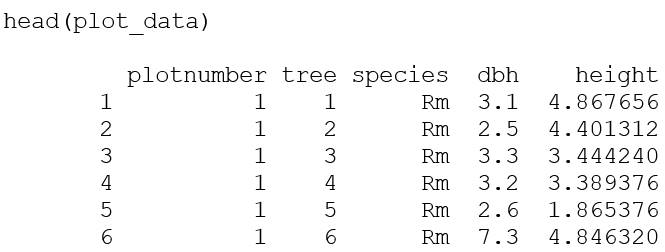
Default column names are “plotnumber”, “species”, “dbh”, “height”. Note that tree number (“tree”) is in the example data set to identify each unique sample, but this column is not required for the function to operate. If your column names are different from the defaults, you can specify them using the appropriate argument (see package help files for more information). Plot numbers are sequential integer values, and the first plot number must be 1. Species can be any meaningful string values; however, DBH must be in centimeters, and height must be in meters. The defaults for both the plot.width and plot.length arguments are 10 m, and the functions assume that each plot is the same area (length × width). A 10 m ? 10-m plot area was chosen as the default, but experience is the best guide to dictate the optimum size of a mangrove structure plot. Common sizes are 5 m ? 5 m for young stands, 10 m ? 10 m in average-age stands, and 10 m ? 50 m or 10 m ? 100 m in mature, developed forests. If unsure what plot size to use, Schaeffer-Novelli and Cintrón (1986) recommend choosing one that will contain from 20 to 30 trees. The plot.method function can also be applied to other common vegetation survey methods, such as those proposed by Dallmeier (1992) and Gentry (1986). To increase sample size, we recommend establishing two or more plots per study site, but the function will run on any number of plots. In usage, the plot numbers are sequential integers, and should begin with 1.
Once the plot data set is properly formatted, the first step is to apply the function plot.method by assigning the function to a new data set in the global environment (in this example “p1” is used). The function calls on the plot data (in the present example, the data set was named “plot_data”) as follows:
p1 <- plot.method(plot_data)
This function will provide a console output with a summary of the plot method analysis, and also will assign a data set to the global environment with the relative computations for later use (such as for graphic display with iv_plot). In the R console, the output looks like this:
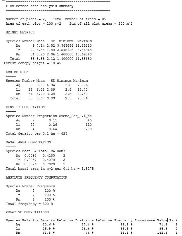
The output begins by summarizing the data set, providing the number of plots, total number of trees, the area of each plot, and the sum of all plot areas. If tree height is provided, height metrics will be displayed, including the canopy height (average of the three tallest trees), mean tree height, standard deviation (SD), as well as the minimum and maximum tree height. Following this, diameter (DBH) metrics are displayed, including mean, standard deviation (SD), minimum, and maximum DBH. Species-level metrics are included for both height and DBH outputs. These include number, mean, standard deviation (SD), and minimum and maximum values.
After the summaries of the data set, the output provides a series of computations, including density, basal area, and absolute frequency. For each computation, there is a breakdown of the species level data, as well as total computations for the data set. Finally, relative computations are provided, summarizing the importance values and rank of each species to the mangrove stand. This final table is also assigned to the global environment (here, “p1”).
The argument for the function plot.method can be modified to accommodate data sets with custom column names or plot sizes. For example, if the column for the plot number is “Plot_Number” (please note that column names are case sensitive), and the plot widths are 20 meters (instead of 10), the argument can be specified as follows:
p1 <- plot.method(plot_data, plotnumber = “Plot_Number”, plot.width = 20)
Note that column names and plot dimensions do not need to be specified in the arguments unless they differ from the default values.
The next available analysis for plot data is the calculation of mangrove forest indices by applying the function plot.indices. This function assumes all the same argument parameters as plot.method with regard to default column names and default plot sizes, and customized values are specified in the same manner as above. The plot.indices function produces an output with two common mangrove forest indices, the complexity index and mean stand diameter. The main purpose of these indices is to capture structural complexity and allow for mangrove forest comparisons across regions (Table 2). The R console output for plot.indices appears as:
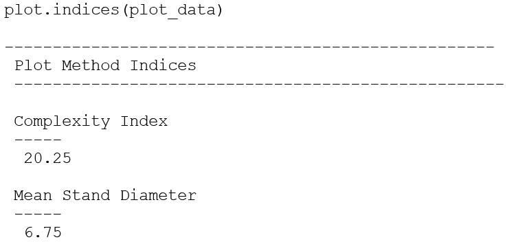
In addition, the plot.indices function provides an optional argument for producing tree size-class bins, based on diameter and height, and one scatterplot depicting the relationship between them. In the usage, if “sizebin = TRUE”, three graphs are generated: (1) an illustration of size class proportions: < 5 cm, 5 cm -10 cm, and >10 cm DBH (Fig. 1A); (2) an illustration of tree height size class proportions: < 5 m, 5 m - 10 m, and >10 m (Fig. 1B); and (3) a scatterplot of the relationship between DBH and height (Fig. 1C). The argument “sizebin = TRUE” allows the user to examine a quick snapshot of the forest structure based on DBH and height. Note that plot.indices does not require assignment to a global environment object.
plot.indicies(plot_data, sizebin = TRUE)
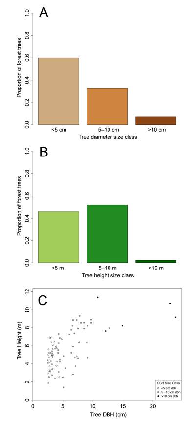
Figure 1. Example outputs from the mangroveStructure package for both plot.indices and pcqm.indices functions (here, test data from plot.indices available from GitHub are shown. In usage of both functions, if “sizebin = TRUE”, three tree size-related graphical outputs are displayed for (A) size class proportions of tree diameters, (B) size class proportions of tree heights, and (C) the relationship between tree diameter and tree height, with diameter size-class color breakdown to aid in visually interpreting forest size structure.
If the user wants to find the fit of a linear model for the height-DBH relationship, they can use the lm function in the base stats package of R. In our example, this would take the form:
summary(lm(plot_data$height ~ plot_data$dbh))
and will output a table with the equation and coefficients of the relationship, as well as estimated fit (i.e., adjusted R2). The user can also subset to one species (i.e., Rhizophora mangle, or “Rm” in the previous example) and find the equation and coefficients for that species. In this case this would take the form:
Rm_data <- subset(plot_data, plot_data$species=="Rm")
summary(lm(Rm_data$height ~ R_data$dbh)
mangroveStructure for plotless data
For the plotless data, the point-centered quarter method (PCQM; Cottam & Curtis, 1956) is utilized. For a review of the point-centered quarter method as applied to mangrove forests, seeCintrón and Schaeffer-Novelli (1984). To illustrate the package for PCQM sampling, mangroveStructure contains the following example taken from a mangrove stand in Darién, Panama. In the output, the species code “A” indicates Avicennia germinans, “L” is Laguncularia racemosa, “M” is Mora oleifera, “PR” is Pelliciera rhizophorae, and “R” is Rhizophora mangle. Akin to the plot functions, the data set must be properly formatted. For PCQM functions, the data set must have four specific columns for plot data analysis: sampling point number, distance, species, and diameter at breast height (DBH). Tree height is an optional column and the function can operate without it; however, when included, additional height-related metrics are calculated and displayed. Note that quarter number is in the example data set to identify each sampling point’s quarter, but this column is not required for the function to operate. Using the R command prompt, head, the user can investigate the dataset (first six rows with column names) to ensure it contains all needed columns, which gives the R output:
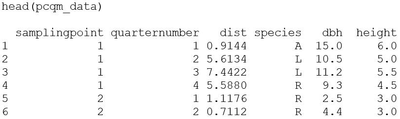
As is the case with the plot method, the accuracy of the PCQM method increases with the number of sampling points (number of trees) surveyed per site. At least 20 sampling points along the transect are recommended by Cottam and Curtis (1956). It is important to emphasize that the PCQM method has two important limitations: (1) an individual tree must be located in each quarter, and (2) an individual tree must not be measured twice (Cintrón & Schaeffer-Novelli, 1984).
Sampling points are sequential integer values, and the first sampling point must be 1. Species can be any meaningful string values, but DBH must be in centimeters and height must be in meters. The default column names are “samplingpoint”, “dist”, “dbh”, “height”. Once the plotless data set is properly formatted, the first step would be to apply the function pcqm.method by assigning the function to a dataset in the global environment object (here, “p2”). The function is applied to the data set (here, “pcqm_data”) as follows:
p2 <- pcqm.method(pcqm_data)
This function will provide a console output with a summary of the PCQM method analysis, and just like the plot function, will assign a data set to the global environment with the relative computations for later use.
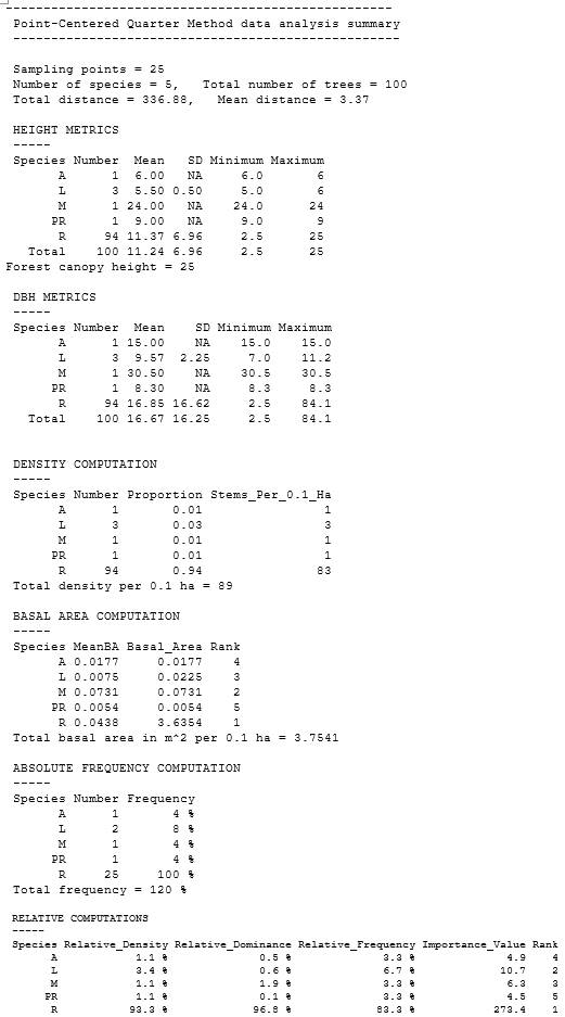
The output here is quite similar to the plot method output. It begins by summarizing the data set, providing the total number of sampling points, number of species, total number of trees, the total distance, and the mean distance from the PCQM measurements. If tree height is provided, height metrics will be displayed, including the canopy height (average of the three tallest trees), mean tree height, standard deviation (SD), as well as the minimum and maximum tree height. Diameter (DBH) metrics are displayed, including mean, standard deviation (SD), minimum, and maximum DBH. Both height and DBH metrics are calculated down to species level.
The remainder of the output is identical to the plot method output. It provides a series of computations, including density, basal area, and absolute frequency. For each computation, there is a breakdown of the species level data, as well as total computations for the data set. Finally, relative computations are provided, summarizing the importance values and rank of each species to the mangrove forest. This table is also assigned to the global environment (here, “p2”).
This function can also be modified to accommodate data sets with custom column names. For example, if the column for the species is “Spp” (please note again that column names are case sensitive), the argument can be specified as follows:
p2 <- pcqm.method(pcqm_data, species = “Spp”)
Note that column names do not need to be specified unless they differ from the default values.
The next available analysis for plotless data is the calculation of mangrove forest indices by applying the function pcqm.indices. This function assumes all the same argument parameters as pcqm.method with regard to default column names, and customized values are specified in the same manner as above. The pcqm.indices function produces an output with two common mangrove forest indices, the complexity index and mean stand diameter:
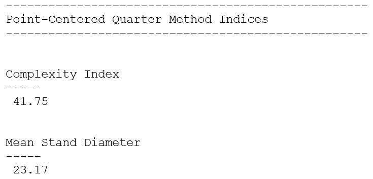
Identical to that for plot data, the pcqm.indices function provides an optional argument for producing graphical size-class bins, based on diameter and height, and one scatterplot depicting the relationship between them. If “sizebin = TRUE”, three graphs are generated: (1) an illustration of size class proportions: <5 cm, 5 cm - 10 cm, and >10 cm DBH; (2) an illustration of tree height size class: < 5 m, 5 m - 10 m, and >10 m, and (3) a scatterplot of the relationship between DBH and height (Fig. 1A-C). This function argument allows the user to examine a quick snapshot of the forest structure based on DBH and height. Note that pcqm.indices does not require assignment to a global environment object.
pcqm.indicies(pcqm_data, sizebin = TRUE)
See table 1 for a description of the pcqm.indices function and table 2 for a description of these indices and their use.
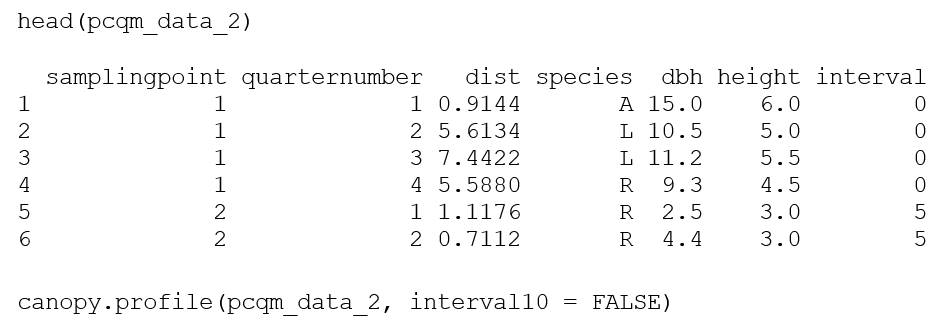
Because PCQM is based on a transect line laid out through the forest, a profile of the forest canopy can be generated. The canopy.profile function will produce a line chart of the forest canopy height using the sampling points and known distances between them (Fig. 2). This function assumes all the same argument parameters as other PCQM functions with regard to default column names, and customized values are specified in the same manner as above.
canopy.profile(pcqm_data)

Figure 2. Example output from the mangroveStructure package canopy.profile function for plotless data (point-centered quarter method) using test data available from GitHub. In this dataset, sampling points were evenly spaced at 10-m intervals (default), however, the function can accommodate custom spacing (see text).
The function has a default assumption of equidistant 10-m spacing between all sampling points. This is specified via the logical argument “interval10”, which is set to the default value TRUE. If the user specifies interval10 = FALSE, a unique column must exist in the data set with distance from the previous sampling point. The default column name for this column is “interval”, which can be specified (“customized”) similar to other column name arguments. For unique interval distances, the first row (sampling point 1) must have a value of 0. Each successive sampling point number represents the distance from the previous sampling point, not the additive distance from sampling point 1. The interval distance must be identical and provided for every tree (all four quarters) at each sampling point.
Importance value radar plots
After running either plot.method or pcqm.method, which assigns to the global environment an object with outputs of the relative computations of density, dominance, and frequency, these data can be graphically summarized via an importance value radar plot (Fig. 3). The iv.plot function creates a radar plot of the top five species (determined by the ranking from the relative importance metrics). The default colors are red, black, blue, yellow, and green; these are assigned to species in alphabetical order. Since common names of many mangrove species are associated with certain colors (e.g., Rhizophora mangle L. is referred to as red mangrove, Avicennia germinans (L.) L. is black mangrove, etc.), colors can be modified by specifying the colors in the function and matching these to the common name of a species. One color must be listed for each species (up to five), which can allow the user to color the species to intuitive values (red mangrove = red, etc.). A convenient source for colors and their corresponding names for R is available online (Colors in R, n.d.), but there are other online resources available. To customize the colors, they should be listed in the alphabetical order of the top five species’ importance values. When using iv.plot, the user must call to the table saved from the output of either plot.method or pcqm.method, as this function cannot be run on raw data. Above in the examples included with the package, these global environment objects were named “p1” and “p2”.
iv.plot(p1, colors = c(“black”, “gray”, “firebrick1”))
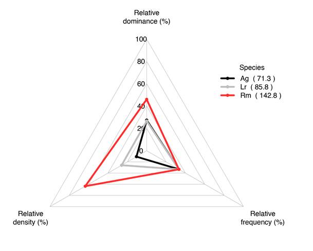
Figure 3 Example of output from the mangroveStructure package iv.plot function for both plot and plotless data depicting radar plot of the top five species (based on importance values) with their relative dominance, density, and frequency. The importance value is displayed in the legend alongside the species names (in parentheses), which are listed alphabetically in the output. Shown are plot test data available for download from GitHub.
Discussion
The mangroveStructure package is an easy and convenient way to process mangrove forest structural data in one easy, convenient package. It implements the most commonly-used metrics employed to describe mangrove stands and offers informative graphic displays to complement the numerical outputs. With the release of this package, the authors hope that mangrove researchers will not only benefit from its convenience, but also, that they will benefit from employing a tool that permits precise management of data for mangrove forest structural attributes. Since mangrove structure and environmental conditions are related (McDonald, Webber, & Webber, 2003; Luo, Sun, & Xu, 2010; Ximenes, Maeda, Arcoverde, & Dahdough-Guebas, 2016), the implementation of this package in mangrove structural surveys would permit a better comprehension of the environmental conditions that underlie mangrove forest structural variability through space and time. It can also aid in the adoption of uniform measurement protocols that can be used for mangrove forest comparisons across regions and time. One of the conveniences of open-source software is that the original code is freely and easily available, and may be modified as needed. In this sense, future work on this package could incorporate additional information based on data gathered with novel methodologies or its modification to work on other forested ecosystems. For instance, a review of stand structural complexity indices was compiled by McElhinny (2005) as they apply to woodland and dry sclerophyll forests in Australia, but few of these indices have been attempted in mangrove forests. While some of these metrics can be easily incorporated into this package, we believe it is best for any structural index to show practical applications in mangrove forest work before it should be coded into the package. In this sense, it is our hope that future versions of this package can be enhanced with input from mangrove researchers around the world.

