


 texto en
  Inglés (pdf)
 Artículo en XML
 Referencias del artículo
 Enviar artículo por email
 Citado por SciELO
  Similares en
SciELO
Similares en
SciELO 
 Permalink
Highlights:
Three machine learning classifiers are evaluated to identify scab and anthracnose diseases in avocado fruits.
The chromatic descriptor extraction technique by region selection was more appropriate than extraction with image subsampling.
The high performance of machine learning classifiers to identify anthracnose and scab in avocado fruits is confirmed.
The classifiers achieved higher performance than a deep learning network applied in a previous study.
Introduction
Mexico is the world's leading producer and exporter of avocado, with production exceeding two million tons in 2021 (Servicio de Información Agroalimentaria y Pesquera [SIAP], 2022); however, postharvest loss is a factor that affects marketing and food security. Two fungal diseases of commercial interest are reported in avocado fruit: scab (Sphaceloma perseae) and anthracnose (Colletotrichum spp.). Improper management of avocado orchards can cause losses of more than 70 % before harvest, and total postharvest losses if environmental and biological conditions exist for the development of these diseases (Téliz & Mora, 2019). Early detection of phytosanitary problems is an essential step to ensure food safety. In the literature, automatic systems with the ability to detect diseases in plant species based on digital images have been proposed (Saleem, Potgieter, & Arif, 2019).
The machine learning (ML) paradigm is widely used to detect diseases. A basic task in ML is the supervised classification or prediction of a discrete response variable. Input data are associated with each target class to form a training set, and the model learns to predict the target classes on an unseen data set (Ketkar & Moolayil, 2021).
In agriculture, different studies have been conducted using ML algorithms for automatic disease detection in plants. Among the paradigms applied are the support vector machine (SVM) (Sandhya, Balasundaram, & Arunkumar, 2022), random forest (RF) (Srinivasa, Venkata, Anusha, Sai, & Bhanu, 2022) and multilayer perceptron (MLP) (Chen, Dewi, Huang, & Caraka, 2020). These algorithms have been applied to different plant organs, such as leaves, roots, or fruits (Doh et al., 2019).
A deep learning classifier allows automatic feature extraction from an input dataset and reduces user error for feature selection. In general, high overall classification accuracy levels are achieved with this approach when large datasets are available. In agriculture, this has been used in disease identification, crop classification, and yield prediction (Alzubaidi et al., 2021).
The aim of this research was to identify anthracnose-infected, scab-infected and healthy fruits (three target classes) by means of three machine learning models (RF, SVM and MLP) and extracted chromatic descriptors (region selection [BD1] and image subsampling [BD2]) from digital avocado fruit images.
Materials and methods
Database
The set of avocado fruit images used in this study (30 per target class) were selected with different disease levels from a database with 569 digital images of 256 x 256 pixels in size, belonging to avocado fruits of the Fuerte variety reported in a previous study (Campos-Ferreira & González-Camacho, 2021) (https://www.kaggle.com/datasets/camposfe1/clasifiacin-de-enfermedades-del-aguacatero).
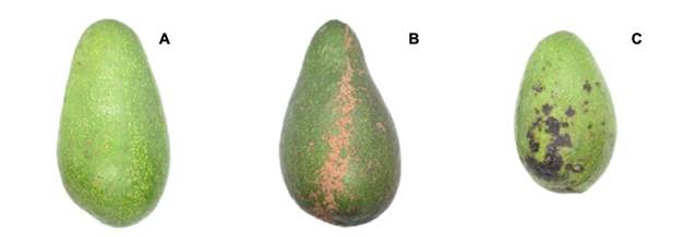
Images of the fruits were captured in the laboratory under homogeneous lighting conditions. The target classes were healthy fruits (H), scab (S, Sphaceloma perseae) and anthracnose (A, Colletotrichum spp.). Fruits were obtained in the municipalities of Ocuituco (18° 51’ 47.6” NL and 98° 46’ 49.1” WL) and Tetela del Volcán (18° 53’ 36.3” NL and 98° 43’ 47.7” WL) in the state of Morelos. Fuerte variety fruits, when ripe, are green, which allows contrasting the lesions caused by the two diseases mentioned (Figure 1).
Software and hardware
Python programming language ver. 3.9 was used as the programming platform, and the scikit-learn ver. 1.0.2 library was used to implement the machine learning classifiers. Training and validation of the classifiers were performed in Spyder development environment ver. 4.2.1 and the MacOs Monterey (12.6) operating system on a Mac mini (Apple) computer, which uses an ARM (M1) chip with 3.2 GHz processing speed and 8 GB of RAM.
Image processing
The set of images represented with the RGB (red, blue and green) color model was transformed to the HSV (hue, saturation and value) color model. This is because the HSV representation is more appropriate than RGB for extracting color features, and allows for improving the performance of learning classifiers (Abdel-Hamid, 2019).
Color feature extraction
The extraction of color features (descriptors) was carried out using two techniques: BD1 and BD2. This was done with the help of the IDENTO program (Ambrosio-Ambrosio, González-Camacho, Rojano-Aguilar, & del Valle-Paniagua, 2023) to create the input datasets from the images for each target class. The BD1 dataset was created using the region extraction technique. This consisted of selecting, in each image, a region of interest, and from a seed, or starting, pixel, the algorithm extracts a set of pixels similar to the seed, where each pixel is represented by the H, S and V color channels. IDENTO allowed generating, for each target class, a set of 45,536 value triplets (H, S and V) (Table 1).
Table 1 Description of the input datasets (pixels or H, S and V color descriptors) obtained with the region extraction (BD1) and image subsampling (BD2) techniques.
| Class | BD1 | BD2 |
|---|---|---|
| H | 15,213 | 17,746 |
| S | 14,836 | 13,416 |
| A | 15,487 | 8,513 |
| Total | 45,536 | 39,675 |
H = healthy fruits; S = fruits with scab; A = fruits with anthracnose.
The BD2 dataset was created using the technique of extraction by subsampling a box-shaped section of the image with the area of interest. For this, with the aid of the IDENTO software, three rectangular areas (30 × 30 pixels) with the representative color of each target class were selected. In total, 90 image samples per target class (270 in total) were obtained; subsequently, the total set of 39,675 value triplets (H, S and V), associated with each target class, was created (Table 1).
In both datasets, repeated triplets within and between target classes were removed. The sets of value triplets (H, S, and V), and their associated target class, were exported and saved to a .csv format file for use in training and testing with the RF classifier.
Random forest (RF)
The RF classifier is a supervised ensemble learning model. In the case of a classification problem, this algorithm uses decision trees based on a condition, and each tree obtains a value to classify the data. Each tree casts a unit vote, and the choice of the best decision tree is made according to the one with the highest number of votes from the entire forest (Parmar, Katariya, & Patel, 2019).
In RF, each tree is constructed from a randomly drawn sample, with replacement, from the training dataset (bootstrap); subsequently, multiple training sets are produced with values other than the initial set. From each sample, a model is built (bagging) and the data from the original sample is inputted, its predicted class is determined and the difference with the actual value is analyzed, thus obtaining the classification error. Ensemble models allow for reducing the variance of the RF estimator and avoiding overfitting of the model (Knauer et al., 2019).
In an RF model, the aim is to maximize the information gain, which is defined by:
where f is the condition dividing the parent node, D p and D j belong to the data of the parent node and the j-th child, I is the impurity metric, N p is the number of samples in the parent node and N j is the number of samples from the j-th child. The information gain is the difference between the impurity of the parent node and the sum of the impurities of the child nodes; the lower the impurities of the child nodes, the greater the information gain (Raschka, Liu, & Mirjalili, 2022).
An objective function used in RF is the Gini criterion (I G ) and is calculated as:
where K corresponds to the number of target classes and
In this work, the random forest classifier function was used, which takes as its main arguments the number of trees (n_estimators, NE), the criterion (criterion, Cr), tree depth (max_depth, MD) and maximum features (max_features, MF) (Raschka et al., 2022). These hyperparameters were used to optimize the RF model based on the following intervals and values (selected by trial and error): NE = 100, 200, 300 and 1000; Cr = ‘gini’ and ‘entropy’; MD = 4, 6 and 8; MF = ‘sqrt’ and ‘auto’.
Support vector machine (SVM)
SVM is a model that associates the data from the original set, from an input space with a high-dimensional feature space, making it simpler in the feature space. This is done to optimally separate the classes in a hyperplane, minimize the generalization error and maximize the margin.
In case the classes are separable from each other from a linear classifier, the SVM model determines the hyperplane that minimizes the generalization error (by means of a test dataset). Otherwise, when at least one class is not separable from the others, SVM tries to find the hyperplane that maximizes the margin and, at the same time, minimizes it by an amount proportional to the number of misclassifications. Based on the selected hyperplane, the maximum margin between classes will be obtained, that is, the sum of the distances between the separation hyperplane and the closest points for each class (Das, Singh, Mohanty, & Chakravarty, 2020).
The equation of a hyperplane is defined as w × x + b = 0, where w is a normal vector to the hyperplane and b is an offset. In the case of a multiclass classification, the following optimization problem is used:
where ξ i (i = 1, …, n) are slack variables, which may allow some data to remove the constraints that define the minimum margin required for the training data for a separable case. C is a user-defined penalty parameter to control the margin of error of the training set; the larger the value of C, the larger the penalty. On the other hand, the j-th SVM is trained with the data in the j-th class with labels belonging to the class, and the other classes with labels different from the class (Pisner & Schnyer, 2020).
There is a kernel function, which is used to transform the training data set so that a nonlinear decision surface is transformed into a linear equation in a larger number of dimensional spaces. In general, this function returns the inner product between two points in a feature dimension. The most commonly used kernels are linear:
And the Radial basis function (RBF) kernel, also known as the Gaussian kernel:
where σ > 0 is the parameter controlling the kernel width. This expression can be simplified as follows:
where
Classification methods are included in the scikit-learn program library, within the svm module. In the present work, the support vector classification (SVC) function was used, which takes as its main hyperparameters the penalty or C value (C), the gamma value (γ) and the kernel mask size (K). By trial and error, the following intervals and values were defined: C = 0.01, 0.1, 1, 10 and 100; γ = 0.001, 0.1, 1, 10 and 100; kernels = ‘rbf ’ and ‘linear’ (Raschka et al., 2022).
Multilayer perceptron (MLP)
In MLP, the basic element is known as an artificial neuron. This artificial neuron, of the feed forward type, consists of input and output elements that are processed in the central unit. The input layers depend on the data used for training, while the hidden layers and the output layers pertain to the number of classes of interest.
The MLP architecture consists of an input layer, one or more hidden layers, and an output layer. The input layer depends on the number of input data, the hidden layers represent the level of complexity that exists between the input and output layer, and the output layer represents the number of target classes and gives the predicted class (Edmond & Girsang, 2020).
The function that transforms the input data is known as the activation function. The most common is the ReLU (Rectified Linear Unit) function, which is expressed as:
where the response is z if the input is positive and 0 if it is negative. ReLU is used to filter the data in the intermediate layers. In the output layer, the softmax activation function is used, which is expressed as:
where p(z) is the probability that an input z belongs to the i-th class (Chollet, 2018).
For MLP training, the adam (Adaptive moment estimation) optimizer was used, which is a variant of the gradient descent method. This method uses the momentum and variance of the loss function’s gradient to update the weights, which allows smoothing the learning curve and improving the learning of the classifier (Géron, 2022).
The scikit-learn neural network module contains the MLPClassifier function, and takes the following hyperparameters as arguments: hidden layer size (HL), number of iterations (It), activation function (AF), optimizer (Op), learning range (LR) and batch size of samples entering the model at each iteration step (BS) (Raschka et al., 2022). The intervals and search values of the hyperparameters were defined by trial and error, and the following were considered: HL = 50, 100 and 500; It = 50, 100 and 500; AF = ‘softmax’ and ’ReLU’; Op = Broyden-Fletcher-Goldfarb-Shanno (lbfgs) and adam algorithm; LR = ‘constant’ and ‘adaptative’; BS = 8, 16 and 32.
Performance metrics
The metrics for determining overall performance and each target class of the classifiers are obtained from the confusion matrix, based on the test data. In the case of a binary classification, this matrix has four possible outcomes: true positive (TP), true negative (TN), false positive (FP) and false negative (FN) (Kulkarni, Chong, & Batarseh, 2020). Based on these values, the following metrics are defined:
Precision (P), which measures how accurate the model is in predicting positive values.
Recall or sensitivity (R), which measures the strength to predict positive outcomes.
The F1 score, which is the harmonic mean between P and R.
These three metrics are used to evaluate the performance of the classifier to predict each class. The evaluation of the overall performance of the classifiers was made based on the overall classification accuracy (ACC) and the area under the curve (AUC) for the ROC (receiver operating characteristic) curve.
ACC is the ratio of correct classifications to the total number of samples, and is expressed as:
The ROC is a graph that is constructed with values for different probability thresholds of the true positive rate (TPR) versus the false positive rate (FPR) (Jiang, Li, & Safara, 2021). AUC varies between 0 and 1, and measures the performance of the model for each target class. TPR is obtained from the following equation:
and FPR is calculated as:
Machine learning model selection
In the literature, it is reported that the RF, SVM and MLP classifiers, in general, achieve good overall classification accuracy (Yuvali, Yaman, & Tosun, 2022). In preliminary tests, these classifiers performed well in terms of classifying avocado fruit images.
Training and testing of classifiers
The training and testing of the classifiers consisted of two stages. In the first, the RF classifier was trained based on the BD1 and BD2 datasets to compare the chromatic descriptor extraction and image subsampling techniques, and to select the one that generates the best RF performance in terms of
Selection of optimal hyperparameters
To optimize each classifier, we first performed a stratified random partitioning by each target class of the dataset at an 80:20 ratio (80 % for training and 20 % for the prediction test). This ratio establishes a balance between the training and test data to measure the performance of the classifiers. The training data were standardized to homogenize the input descriptors using the following expression:
where x corresponds to each descriptor of the input set, µ x is the mean of the set of x values and σ x is the sampling variance of the set of x values.
Optimal hyperparameter selection was performed using a grid search and cross-validation with k = 10 disjoint groups. For each classifier, value intervals of each hyperparameter were defined to select the combination of values that maximize the average ACC of the classifier (Liashchynskyi & Liashchynskyi, 2019).
Cross-validation consists of dividing the training set randomly into k disjoint groups, where k-1 groups are used as training sets, and the remaining group as a validation set. This process is repeated k times for each combination of hyperparameter values, and an average ACC of k model runs is obtained (Raschka et al., 2022). The optimal combination of hyperparameter values is the one that generates the maximum average ACC value.
Classifier prediction test
With the set of optimal hyperparameters obtained in the training stage, a cross-validation procedure was performed with k = 10 groups with the total input dataset (100 %) to recalculate the weights or parameters of each classifier. In each k run, the ACC prediction performance was determined for each k-th test set. After k runs, the average ACC performance of each classifier was obtained.
The codes implemented for the present work can be found at the following link: https://github.com/Camposfe1/Avocado-disease-classification.git.
Results and discussion
Selection of optimal hyperparameters
The optimal hyperparameter values for each classifier were NE = 10, MF = ‘auto’, MD = 8 and Cr = ‘entropy’ for RF, C = 10, γ = 10 and K = ‘rbf’ for SVM, and BS = 8, HL = 150, AF = ‘ReLU’, It = 100 and Op = ‘adam’ for MLP.
Comparison of descriptor extraction techniques
Comparison of color feature or descriptor extraction techniques, by region and image subsampling, as well as their effect on RF classifier performance, showed that selection by region (BD1) allows generating color pixel sets with more information to differentiate the three target classes (H, S and A). RF obtained greater accuracy to classify the three target classes. The values of FP and FN, for each class, were lower than those corresponding to BD2. Likewise, extraction by region generated better balanced class sizes than by subsampling (Figure 2).
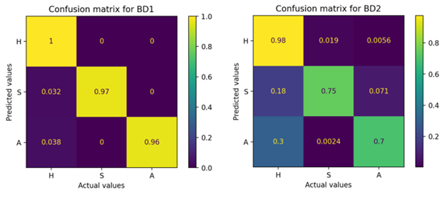
Figure 2 Confusion matrices of the random forest (RF) classifier based on the datasets generated with region extraction (BD1) and image subsampling (BD2). Target classes: H = healthy fruit; S = fruit with scab; A = fruit with anthracnose. Predicted versus actual color pixels by target class.
Similarly, RF performance, overall and at the class level, was superior with BD1 than with BD2. With BD1, RF achieved an average ACC of 98 %, while with BD2 it was 84 %. At the class level, F1 scores were higher than 97 % with BD1 and higher than 76 % with BD2 (Table 2).
Table 2 Prediction performance metrics of the random forest (RF) classifier based on region-based color descriptor extraction (BD1) and image subsampling (BD2) methods.
| Metric | BD1 | BD2 | ||||||
|---|---|---|---|---|---|---|---|---|
| H | S | A | H | S | A | |||
| P | 0.94 | 1.00 | 1.00 | 0.77 | 0.97 | 0.76 | ||
| R | 1.00 | 0.97 | 0.96 | 0.98 | 0.75 | 0.84 | ||
| F1 | 0.97 | 0.98 | 0.98 | 0.86 | 0.84 | 0.76 | ||
| AUC | 1.00 | 1.00 | 1.00 | 0.97 | 0.94 | 0.95 | ||
| ACC | 0.98 ± 0.03 | 0.84 ± 0.08 | ||||||
H = healthy fruits; S = fruits with scab; A = fruits with anthracnose; P = precision; R = recall; F1 = F1 score; ACC = overall classification accuracy; AUC = area under the ROC curve.
Evaluation of the prediction of RF, SVM and MLP classifiers
The prediction performance of the three classifiers was high. The confusion matrices for each classifier show that RF and MLP achieved the highest ACC for all three classes. All three classifiers have the highest FP value for predicting class H; that is, the classifiers predict samples from classes S or A as H. For this analysis, there are pixel samples with scab that are predicted to be healthy, and healthy samples that are predicted to have anthracnose (Figure 3).
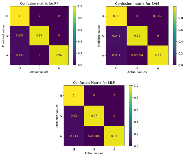
Figure 3 Confusion matrices of the random forest (RF), support vector machine (SVM) and multilayer perceptron (MLP) classifiers based on descriptor extraction by region (BD1). Target classes: H = healthy fruits; S = fruits with scab; A = fruits with anthracnose.
In terms of overall classifier performance, RF and MLP were superior to SVM with an ACC of 98 %. Likewise, both classifiers obtained an F1 score above 97 % for each target class (Table 3).
Table 3 Prediction performance metrics of random forest (RF), support vector machine (SVM) and multilayer perceptron (MLP) machine learning classifiers based on descriptor extraction by region (BD1).
| Metric | RF | SVM | MLP | ||||||||
|---|---|---|---|---|---|---|---|---|---|---|---|
| H | S | A | H | S | A | H | S | A | |||
| P | 0.94 | 1.00 | 1.00 | 0.94 | 1.00 | 0.99 | 0.95 | 1.00 | 1.00 | ||
| R | 1.00 | 0.97 | 0.96 | 0.99 | 0.95 | 0.97 | 1.00 | 0.97 | 0.97 | ||
| F1 | 0.97 | 0.98 | 0.98 | 0.96 | 0.98 | 0.98 | 1.00 | 0.98 | 0.98 | ||
| AUC | 1.00 | 1.00 | 1.00 | 0.99 | 0.99 | 0.99 | 0.99 | 0.99 | 1.00 | ||
| ACC | 0.98 ± 0.03 | 0.97 ± 0.06 | 0.98 ± 0.03 | ||||||||
H = healthy fruit; S = fruit with scab; A = fruit with anthracnose; P = precision; R = recall; F1 = F1 value; AUC = area under the ROC curve; ACC = overall classification accuracy.
The BD1 method of extracting features or color descriptors had a significant effect on classifier performance. This method allowed obtaining pixels or color samples representative of each target class and balanced class sizes, which led to better classifier performance. The BD2 feature extraction method generated a dataset with unbalanced classes and the H class of healthy fruits was favored. The imbalance between class sizes in BD2 had a negative effect on the performance of the RF classifier, which reached an ACC of 84 %. Some publications state that there is no difference between feature extraction methods (Jones, Faiz, Qiu, & Zheng, 2022; Suresh & Mohan, 2020); however, in this study the BD1 selection technique allowed obtaining a better ACC of the RF model than BD2, which depends on the ability to select the areas of interest (Chen et al., 2020). In the case of unbalanced classes, the F1 metric (harmonic mean of P and R) is a more suitable measure to evaluate classifier performance (Fourure, Javaid, Posocco, & Tihon, 2021).
When there are unbalanced classes, the classifiers bias the prediction to the majority class; hence, there is a misclassification for the minority class (Kaur, Singh, & Kaur, 2019). This is because it is easier to get healthy fruits than ones with disease symptoms, since certain conditions are needed for symptoms to be expressed in the fruit (Wardhani, Rochayani, Iriany, Sulistyono, & Lestantyo, 2019).
The three classifiers, RF, SVM, and MLP, categorized scab and anthracnose fruit with an F1 score of 98 %, and were the best-classified classes. Fruits with scab are visually differentiated from healthy or anthracnose fruits; therefore, pixel values between classes are more contrasting.
The machine learning classifiers used in this study show that high performance levels can be achieved with small datasets and shorter computational times compared to deep learning classifiers, particularly convolutional neural networks, which require longer computational times. However, in more complex identification problems, with a large number of classes (greater than 10) and large datasets (thousands of images), deep learning algorithms are more appropriate (Alzubaidi et al., 2021).
Conclusions
The extraction of color descriptors with the region selection method induced a better overall classification accuracy (ACC = 98 %) of the random forest classifier, in contrast to the image subsampling extraction method (ACC = 84 %). All three classifiers (random forest, vector support machine and multilayer perceptron) obtained a ACC greater than 97 % for classifying the surface of avocado fruits as being healthy, with scab or with anthracnose. Likewise, the fruit surface classes with scab and with anthracnose obtained an F1 score of 98 % with all three classifiers.

