


 text in
  English (pdf)
 Article in xml format
 Article references
 Send this article by e-mail
 Cited by SciELO
  Similars in
SciELO
Similars in
SciELO 
 Permalink
Introduction
According to Grijalva-Contreras, Macías-Duarte, and Robles-Contreras (2011), annual greenhouse yields of 24 tomato hybrids in the Caborca region of Mexico ranged from 26.7 to 31.1 kg·m-2, while in the United Kingdom up to 52.6 kg·m-2 per year are reported (Antón et al., 2012). An important element to raise the yields and quality of agricultural products in greenhouses is the control of climate variables, so it is necessary to know the behavior of those factors that directly affect them.
López-Cruz and Hernández-Larragoiti (2010) have described black box models that accurately predict variables such as temperature and relative humidity within a greenhouse, in which they apply neurodiffuse models with R2 between 0.95 and 0.97. Likewise, Salazar-Moreno, López-Cruz, Rojano, Schmidt, and Dannehl (2015) used a dynamic neural network model to predict tomato yields in a semi-closed greenhouse with good performance, reflected by an R2 of 0.97. However, this type of model has the disadvantage of not including information on mass and energy transfer processes, nor on the parameters that intervene in them; contrary to the dynamic models of the climate inside the greenhouse, which also provide information on the heat exchange processes.
The energy balance within greenhouses includes all modes of heat transfer (by thermal radiation, conduction and convection), as described in the models used by Al-Jamal (1994), Arinze, Schoenau, and Besant (1984), Baille (1999), Boulard and Baille (1987), Kindelan (1980), Rodríguez, Berenguel, Guzman, and Ramírez-Arias (2015), van Beveren, Bontsema, van Straten, and van Henten (2015a y 2015b) and Walker (1965). The first component of the energy balance is the solar radiation that falls on the greenhouse cover, which can be transmitted, reflected or absorbed. The proportion of radiation that passes through the cover is known as transmissivity, and depends on the characteristics of the greenhouse cover and the type of radiation (direct or diffuse) (Hernández, Escobar, & Castilla, 2001). The cover isolates the internal atmosphere from outside climate conditions, so it acts as a link between both environments (Rodríguez et al., 2015). Another component of the energy balance is ventilation (natural or forced), which prevents excessive heating during the day, ensures minimum CO2 levels and controls humidity (Castilla-Prados, 2007).
On the other hand, plant transpiration causes heat loss in the greenhouse, which depends on water vapor concentration, transpiration conductance, leaf area index, net crop radiation and stomatal resistance that limits transpiration (Bakker, Bot, Challa, & Braak, 1995). Water vapor condensation in greenhouses, although not very large, constitutes another loss of heat to be considered in the energy balance, as well as that through the soil, which constitutes nearly 10 % of total losses (Rodríguez et al., 2015).
By knowing the outside climate variables (air temperature, wind speed and solar radiation), the properties of the cover and the crop and greenhouse specifications, a set of differential equations can be stated and solved simultaneously in order to describe the behavior of the air temperature inside the greenhouse with respect to time.
Based on the above, the objectives were: 1) to develop a dynamic energy balance model to predict the air temperature inside an experimental greenhouse with tomato cultivation, located at the Universidad Autónoma Chapingo, Mexico, b) to obtain the optimal values of the main parameters involved in the heat transfer processes through the calibration of the model, and c) to evaluate the model for its use as a tool to optimize energy consumption in heating systems and control the greenhouse climate.
Materials and methods
Crop management
The study was conducted at the Universidad Autónoma Chapingo, Mexico, located at 19° 29’ LN, 98° 53’ LW and at an altitude of 2,240 m, for which we used a greenhouse 8 m wide by 15 m long (120 m2), with polyethylene cover, anti-insect netting, two side windows (6 m wide by 13 m long), a zenithal window (15 m long by 1 m wide) and a manual opening and closing system.
The commercial tomato (Solanum lycopersicum L.) hybrid "El Cid", of undetermined habit and saladette-type fruit, was used. Sowing was carried out on March 6, 2016 in 200-cavity polystyrene trays with peat moss as substrate, and on April 24 the seedlings were transplanted into volcanic sand substrate with a density of 3.5 plants·m-2. They were fertilized with Steiner nutrient solution (Steiner, 1961) and tutoring was carried out according to crop needs. Pollination was done manually 15 days after transplant (dat) and the harvest started 125 dat.
For the measurement of climate variables, two HOBO weather stations were installed (Figure 1), one inside the greenhouse to record the inside temperature, soil temperature, global radiation and relative humidity. The sensors were placed in the center of the greenhouse and measurements were carried out every minute. In the case of roof temperature, two sensors were installed on the cover and the data were stored every minute in a data acquisition system (datalogger). In addition, an anemometer was placed on the outside of the greenhouse 2.5 m from the ground to measure wind speed.

Dynamic energy balance model
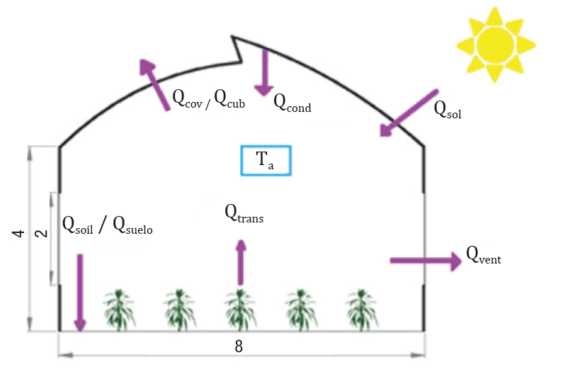
The dynamic energy balance model is based on the models described by de Zwart (1997), van Beveren et al. (2015a and 2015b), van Henten and Bontsema (2009), van Ooteghem (2010) and Vanthoor, van Henten, Stanghellini, and de Visser (2011). Figure 2 shows the state variable air temperature (Ta), the inputs (heat gain due to solar radiation [Q sol ] and heat gain due to water vapor condensation on the roof [Q cond ]; both in W·m-2) and system outputs (heat loss through the cover [Q cov ], heat loss due to ventilation [Q vent ], heat loss through crop transpiration [Q trans ] and heat loss through the soil [Q soil ]; all in W·m-2).
Likewise, Figures 3 and 4 show the behavior of the dynamic model’s input variables for 68 days (99,158 data in total), corresponding to the final tomato growth period (from June 18 to August 26, 2016).
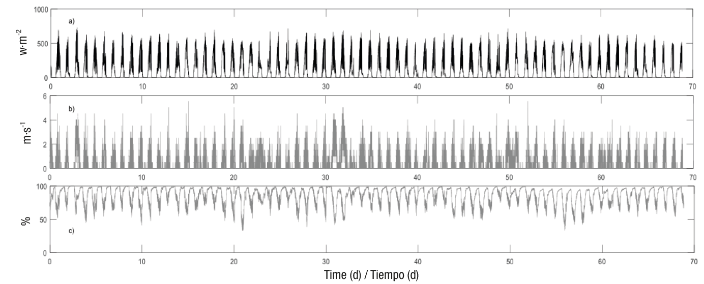
Figure 3 a) Solar radiation (inside), (b) wind speed (outside) and (c) relative humidity (inside), from June 18 to August 26, 2016 (68 days).
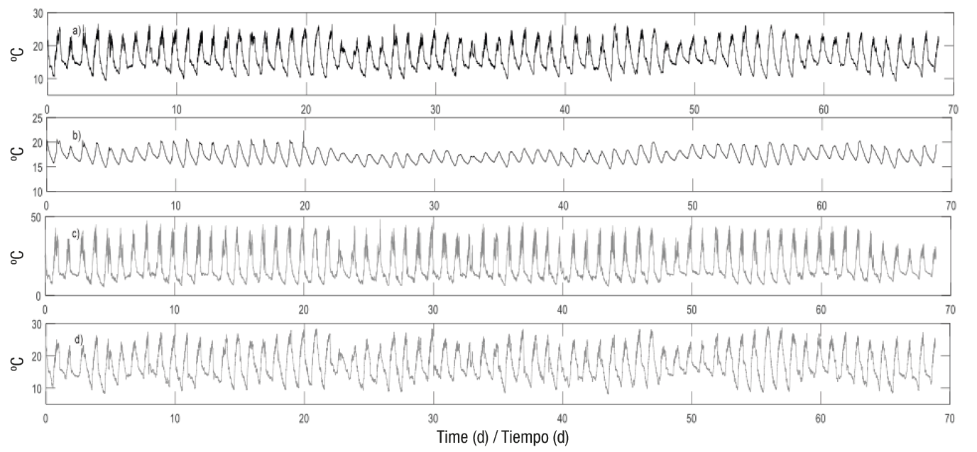
Figure 4 a)Temperature inside the greenhouse, (b) soil temperature, (c) cover temperature and (d) external temperature, from June 18 to August 26, 2016 (68 days).
The non-stationary state energy balance model for air temperature is given by the following ordinary differential equation, where the independent variable is time (t) and the dependent variable is the temperature of the air (Ta):
If the energy flows per unit area (W·m-2) are considered, Equation (1) is modified and instead of the volume (V, m3) we have h:
where
Table 1 Value of the parameters used in the simulation.
| Symbol | Description | Units | Value |
|---|---|---|---|
| V | Greenhouse volume | m3 | 630.00 |
| As | Greenhouse floor area | m2 | 120.00 |
| Ac | Cover area | m2 | 345.30 |
| Avent | Ventilation area | m2 | 171.00 |
| l0 | Window length | m | 3.20 |
| w0 | Window width | m | 0.80 |
| ps | Depth at which soil temperature is estimated | m | 0.05 |
| Cp | Specific heat of the air | J·kg-1·oC-1 | 1000.00 |
| ρ | Air density | kg·m-3 | 1.22 |
| αc | Heat transfer coefficient of the cover | W·m-2·°C-1 | 5 |
| τtot | Solar radiation transmission coefficient | - | 1 |
| ks | Heat transfer coefficient through soil | W·m-1·°C-1 | 5.75 |
| k | Crop-specific transpiration parameter | - | 0.40 |
| kpo | Mass transfer coefficient | m·s-1 | 0.002532 |
| rb | Aerodynamic resistance | s·m-1 | 200 |
| λ | Latent heat of vaporization | KJ·kg-1 | 2,500 |
| LAI | Leaf area index | cm2·cm-2 | 2.2 |
| P | Atmospheric pressure | m·s-2 | 98.1 |
| F 0 | Pressure loss coefficient | - | |
| Cf | Infiltration coefficient | m3·s-1·m-2 | 0.008361 |
| Cd | Discharge coefficient | - | 0.6497 |
| Cw | Wind effect coefficient | - | 0.14 |
Table 2 Energy balance variables.
| Symbol | Description | Units |
|---|---|---|
| Irad | Outside solar radiation | W·m-2 |
| Qsol | Heat gain due to solar radiation | W·m-2 |
| Qcond | Heat gain due to condensation | W·m-2 |
| Qcov | Heat gain through the cover | W·m-2 |
| Qtrans | Heat gain due to crop transpiration | W·m-2 |
| Qsoil | Heat loss through the soil | W·m-2 |
| Qvent | Heat loss due to ventilation | W·m-2 |
| φcond | Condensation conductance | kg·s-1 |
| Rn | Net radiation at crop level | W·m-2 |
| Ta | Inside temperature | °C |
| Tc | Cover temperature | °C |
| Ts | Soil temperature | °C |
| Te | Outside temperature | °C |
| RHe | Outside relative humidity | % |
| RHin | Inside relative humidity | % |
| Xcul | Absolute water vapor concentration in the crop | kg·m-3 |
| X | Water vapor concentration in the greenhouse | kg·m-3 |
| Xsat | Saturated water vapor concentration | kg·m-3 |
| ɛ | Ratio of the latent to sensible heat content of saturated air | - |
| GE | Transpiration conductance | m·s-1 |
| ϕcond | Condensation flow | kg·s-1 |
| rs | Stomatal resistance | s·m-1 |
| ve | Outside air velocity | m·s -1 |
| Tsv | Infiltration rate per unit floor area | m3·m-2·s-1 |
| Tv | Ventilation rate per unit floor area | m3·m-2·s-1 |
| t | Time | s |
On the other hand, Q sol can be expressed as:
Since solar radiation was measured inside the greenhouse, the value of 1 was taken for the solar radiation transmission coefficient (τ tot ), while Q cov is based on the model of van Beveren et al. (2015b) (Equation 4).
The model proposed by Stanghellini and Jong (1995) was used to calculate the greenhouse tomato Q trans :
where the latent heat value of vaporization (λ) reported by Monteith and Unsworth was considered (λ = 2,500 J·g-1), whereas transpiration conductance (G E ) (van Beveren et al., 2015b), ratio of latent to sensible heat content of saturated air (ε), stomatal resistance parameter (r s ) and net radiation (R n ) at crop level (Bontsema et al., 2007) are given by the following equations:
The water vapor concentration in the crop (X cul ) and the saturated vapor concentration (X sat ) in Equations 10 and 11, respectively:
On the other hand, the Q vent was obtained with the equation described by Ruiz-García, López-Cruz, Arteaga-Ramírez, and Ramírez-Arias (2015):
where the ventilation rate (T v ; Baeza et al., 2014) and the discharge coefficient (C d ; Ruiz-García et al., 2015) are given by:
Replacing the window width and length values gives a value of C d = 0.6497. In terms of the wind effect coefficient (C w ), Ruiz-García et al. (2015) report a value of 0.16 for a greenhouse with an area of 2,565 m2, while Roy, Boulard, Kittas, and Wang (2002) and Valera, Molina, and Álvarez (2008) present a value of 0.14 for a 179 m2 greenhouse, which was used in this work.
The first part of Equation 13 is ventilation through windows, while the second part is ventilation due to leakage from the greenhouse construction, or infiltration rate (Ts v ):
The heat gain due to condensation was obtained with the equation of Speetjens, Stigter, and van Straten (2010):
where the condensation conductance (φ cond ) was calculated as follows:
For this equation, the mass transfer coefficient (k po ) determines the condensation rate, and the X sat and the water vapor concentration in the greenhouse (X) are given by:
For the conversion of relative to absolute humidity, the expression proposed by Blasco, Martínez, Herrero, and Ramos (2007) (Equation 20) was used, which is a function that ensures that relative humidity will never be greater than 100 %.
Finally, the Q soil was estimated with the equation of de van Ooteghem (2010). The depth at which soil temperature was estimated was 0.05 m in the first soil layer:
The MATLAB/SIMULINK programming environment was used to generate the computational model. This consists of a main program where parameters are defined (input and output variables, as well as simulation options) and a C-MEX file (S-function) where the model equations are implemented, which is called by a SIMULINK mdl file. The numerical simulation was performed with the Runge-Kutta 4th order integration method, known as Matlab’s ode45 function Dormand-Prince method, with step size of variable integration, and relative and absolute tolerance of 1x10⁻⁸ and 1x10⁻¹⁰respectively. A total of 99,158 data were available to construct, calibrate, and evaluate the model.
Calibration
Calibration of a model is the process of altering the parameters to obtain a better fit of the model with respect to the measured data; in addition, it is a non-linear optimization problem, where the objective is to minimize the mean square error (MSE) between the measured variable (y i ) and the simulated one (ŷ i ), which is subject to the lower and upper limits of the parameters:
where L Ipi and L Spi are the lower and upper limit of the value of the model parameters, respectively, and pi is the i-th parameter with i = 1, …, n.
The nonlinear least squares procedure (Matlab lsqnonlin function) was used to calibrate the parameters.
Fit measurements
In order to know the accuracy of the model’s prediction in relation to the measured variables, we used the MSE, mean absolute error (MAE), root mean squared error (RMSE), root mean absolute error (RMAE) and efficiency (EF) (Equations 23 to 27) (Wilks, 2011). The last statistical measure is one of the most important to determine the model’s behavior. On the other hand, the MSE, when calculated with squared prediction errors, is more sensitive to large deviations and outliers; therefore, an alternative to determine the error of the model is the MAE, which like the MSE avoids the compensation between the under or over prediction (Wallach, Makowski, Jones, & Brun, 2013).
If the model is perfect, the predicted values will be equal to those observed or measured (y i = ŷ i ); therefore, the model’s efficiency will be 1. On the contrary, a model with EF = 0 means that the predicted value is equal to the mean and the second part of Equation 27 is equal to 1, so it will not be a good model. If EF < 0, it means that the predictor is a worse estimator than the mathematical expectation. The fit measures were used both in the estimation of model parameters (calibration) and in the evaluation stage.
Results
The climate variables, both inside (air, floor and roof temperatures, solar radiation, relative humidity) and outside (temperature and wind speed), were obtained every minute. Of a total of 99,158 available data, 48 % (47,997 data, from June 18 to July 22, 2016) were used to construct and calibrate the model, and 52 % (51,153 data, from July 22 to August 26, 2016) to evaluate it.
The model’s simulation results for the air temperature inside the greenhouse were compared with the observed data (Figure 5). In addition, different statistical fit measures were obtained (Table 3) to determine the closeness between the air temperature measurements and the dynamic model’s predictions.

Figure 5 Comparison between the air temperature measured inside the greenhouse and that simulated by the model before calibration.
Table 3 Fit measurements between measured and simulated temperature by the model.
| Fit measurements | Before calibration | After calibration | Model evaluation |
|---|---|---|---|
| MSE1 | 5.0887 | 1.51 | 1.8006 |
| RMSE | 2.2558 | 1.23 | 1.3419 |
| MAE | 1.8641 | 0.99 | 1.0894 |
| RMAE | 0.1118 | 0.097 | 0.0646 |
| EF | 0.6571 | 0.89 | 0.8674 |
1MSE = mean square error; RMSE = root mean squared error; MAE = mean absolute error; RMAE = root mean absolute error; EF = efficiency.
In the model developed, eight parameters are related to greenhouse dimensions (V, A s , A c , A vent , l 0 , w 0 , p s , F 0 ) and four are constant (C p , ρ, λ, P); also, the τ tot was equal to 1, since the solar radiation was measured inside the greenhouse. Due to the above, the sensitivity analysis was not performed, so the model was directly calibrated to improve its performance with the remaining parameters: aerodynamic resistance (r b ), heat transfer coefficient of the cover (α c ), soil heat exchange coefficient (k s ), crop-specific transpiration parameter (k), infiltration coefficient (C f ) and wind effect coefficient (C w ). The initial values of these parameters were obtained from the literature (Table 4), which were varied in different percentages with respect to the nominal values. The range of variation that generated the best results is shown in Table 4.
Table 4 Nominal value and variation of the parameters to be calibrated.
| Nominal value | Reference | Variation range | Optimal values after calibration |
|---|---|---|---|
| Cf 1 = 0.008361 | Ruiz-García et al. (2015) | 0.00418 < Cf < 0.0125 | Cf = 0.0125 |
| αc = 5 | van Beveren et al. (2015b) | 1 < αc < 10 | αc = 10 |
| rb = 200 | Bontsema et al. (2007) | 100 < rb < 300 | rb = 300 |
| ks = 5.75 | Leal (2008) | 1 < ks < 20 | ks = 1 |
| k = 0.4 | van Beveren et al. (2015b) | 0.008 < k < 0.6 | k = 0.008 |
| Cw = 0.14 | Valera et al. (2008) Roy et al. (2002) | 0.05 < Cw < 0.2 | Cw = 0.2 |
1Cf = infiltration coefficient; αc = heat transfer coefficient through the cover; rb = aerodynamic resistance; ks = heat transfer coefficient through soil; k = crop-specific transpiration parameter; Cw = wind effect coefficient.
Model performance improved substantially after calibration (Figure 6 and Table 4), where the percentage change in the decrease of MSE, AME, RMSE and RMAE was 70.32, 46.89, 45.47 and 13.23 %, respectively, and the percentage change in increased efficiency was 35.44 %.
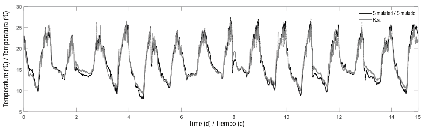
Figure 6 Comparison between the air temperature measured inside the greenhouse and that simulated by the model after calibration.
Once calibrated, the developed model can be used as a black box to test its performance with different information; that is, it also predicts responses when fed with new information. This is known as model evaluation, which was implemented with 52 % of the data (Table 4 and Figure 7). On the other hand, the energy balance model predicts in an acceptable way the variation of the air temperature inside the greenhouse.

Discussion
In relation to the results of the model calibration, the value of the parameters (Table 3) was compared with the results obtained by other researchers. The value of the r b found is higher than the typical one suggested by Bontsema et al. (2007) for a Dutch greenhouse with tomato cultivation (r b = 200 s·m-1), but is similar to that obtained by Qiu et al. (2010) for tomato in a solar greenhouse in China (r b = 295 s·m-1).
The C w depends on greenhouse dimensions and wind speed, so after calibration a slightly higher value (C w = 0.2) was obtained than that found by Ruiz-García et al. (2015) (C w = 0.16) for a polyethylene greenhouse with tomato cultivation. However, it is within the range of values reported by Molina-Aiz, Valera, Peña, Gil, and López (2009) (between 0.16 and 0.82). Likewise, the C f was higher (0.0125 m3·s-1·m-2) than that obtained by Ruiz-García et al. (2015), which means that the model overestimates the infiltration rate.
On the other hand, the α c is higher (10 W·m-2·°C-1) than that reported by the Food and Agriculture Organization of the United Nations (FAO, 2002) for plastic (between 6 and 8 W·m-2·°C-1) and glass (8.8 W·m-2·°C-1) greenhouses, while the optimal value found for the k s (1 W·m-1·°C-1) is equal to that reported by Valera et al. (2008) for dry soil, and is within the range of the values obtained by Abu-Hamdeh and Reeder (2000) for sandy soil (between 0.58 and 1.94 W·m-1·°C-1) and sandy loam soil (between 0.19 and 1.12 W·m-1·°C-1). Finally, the k was lower than the level proposed by van Beveren et al. (2015b), which implies that more research is needed to determine the role of this parameter, by using a value close to nominal (reported in the literature), on the quality of the model prediction.
The under and overestimation of the parameters can be attributed to the fact that in the construction, calibration and evaluation of the model, the ventilation area was considered constant, since the greenhouse was open most of the time; only the vents were closed in rainy weather from 7:00 pm to 8:00-8:30 am. The latter was not considered in the model, and its inclusion could improve its performance. In addition, the leaf area index was considered constant, but its inclusion as an input variable could improve the estimation of transpiration.
As for the approach of the model as a single energy balance equation for estimating the temperature inside the greenhouse, it is considered that it can be improved by including non-stationary state balances at the cover, plant and soil level, and by using a system of ordinary differential equations and not just an equation in the balance. That is, carrying out balances in several layers within the greenhouse environment (de Zwart, 1997). Likewise, the quality of the prediction for the air temperature inside the greenhouse can be improved by considering the balance of matter associated with air humidity. However, if a simple model is generated (with few state variables), it can easily be used in optimizing and controlling the greenhouse environment (Seginer, van Straten, & van Beveren, 2017a y 2017b; van Beveren et al., 2015a and 2015b).
Conclusions
An energy balance model was developed to predict the air temperature inside the greenhouse and the main parameters influencing the thermal behavior of the greenhouse were identified and calibrated. The results obtained after calibration substantially improved the model's performance. The fit measurements indicate a model with efficiencies of 89 and 86 % after calibration and in model evaluation, respectively.
Although the crop-specific transpiration parameter (k) is not very close to the values reported in the literature, the model, in general, has an adequate performance and can be used as a support tool to analyze the temperature behavior inside a greenhouse under different conditions in the central region of Mexico.

