


 text in
  English (pdf)
 Article in xml format
 Article references
 Send this article by e-mail
 Cited by SciELO
  Similars in
SciELO
Similars in
SciELO 
 Permalink
Introduction
The strawberry is a fruit with a high content of vitamins and minerals. It helps to lower cholesterol and its organic acids have disinfectant and anti-inflammatory effects. In Mexico, it is the thirteenth biggest export product and ranks third in the value of Mexico's exports (Servicio de Información Agroalimentaria y Pesquera [SIAP], 2016).
The world’s leading strawberry producer is mainland China with 2,997,504 t, followed by the United States with 1,360,869 t, Mexico with 489,198 t, Turkey with 372,498 t, Spain with 312,500 t, Egypt with 254,921 t and the Republic of Korea with 216,803 t (Organización de las Naciones Unidas para la Alimentación y la Agricultura [FAO], 2013).
The US is the leading strawberry consumer worldwide. Its imports in 2013 were 1,499,414 t fresh weight, followed by Canada with 123,384 t, Germany with 112,105 t, France with 929.67 t and Russia with 571,75 t (FAO, 2013).
The main strawberry producing states in Mexico, in order of declining importance, are: Michoacán, Baja California, Jalisco, Baja California Sur and the State of Mexico. Michoacán produces more than 60 % of total domestic production, and it showed a 27 % increase for the period 2005 to 2014 (SIAP, 2014).
In 2014, Michoacán produced 259,190 t in 5,896 ha, equivalent to a yield of 43.96 t∙ha-1. The state is divided into three producing regions: Zamora Valley, Panindícuaro Valley and Maravatío Valley (SIAP, 2014). Domestic production for 2014 was 430,403.43 t; of this, only 158,242.23 t were exported, representing 37 % of total production (SIAP, 2014).
The aim of this research was to analyze the potential for strengthening strawberry exports from Michoacán to the United States, assuming the possibility of increasing exports of this product from the state. To this end, a study was conducted of the strawberry production growth rate (area and yield) and a forecast was made for strawberry exports from Mexico to the U.S. The price elasticities of supply and demand were calculated using logarithmic models, under the assumption that strawberry production in Michoacán grows more because of the increase in yield than the increase in planted area.
Materials and methods
In order to identify the characteristics of the production process, documentary and field information was used, as well as interviews with producers, authorities and representatives of associations, using a completely randomized method.
In order to identify the share of the production increase due to changes in the planted area and those resulting from increases in yield, it was used an exponential function of the type 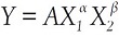 , where: Y is production in t fresh weight, X
1
is planted area, X
2
is yield per ha, α is the relative growth rate of the planted area and β is the relative growth rate of yield, from 2005 to 2014. The planted area was considered because in the evaluated period there was very little or no change in the harvested area (the difference between the two measures was 1.37 %).
, where: Y is production in t fresh weight, X
1
is planted area, X
2
is yield per ha, α is the relative growth rate of the planted area and β is the relative growth rate of yield, from 2005 to 2014. The planted area was considered because in the evaluated period there was very little or no change in the harvested area (the difference between the two measures was 1.37 %).
The strawberry export forecast was made up to 2020 to determine changes in the growing trend towards the U.S., with data validated from 1990 to 2013. The data showed an upward slope. A cubic function of the form Exp = a 0 + a 1 T + a 2 T 2 + a 3 T 3 was proposed, where: Exp = exports, T = year, in order to observe if exports will continue with the same trend or if there will be any change or stagnation in the near future.
For Mexico, field and database information was obtained from: Servicio de Información Agroalimentaria y Pesquera (SIAP), Banco de México, Instituto Nacional de Estadística y Geografía (INEGI), Secretaría de Agricultura, Ganadería, Desarrollo Rural, Pesca y Alimentación (SAGARPA, 2012, 2010 and 2005), Sistema de Información Arancelaría Vía Internet (SIAVI, 2016), among others. Monthly information for the period from 2000 to 2014 was used, while for the U.S., annual data from 1980 to 2014 were used. The study periods correspond to the information validated during the research.
For the partial equilibrium analysis, several logarithmic models were performed until obtaining the one that best explains supply and demand.
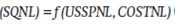
For the U.S. strawberry supply, the variables tested were: production, producer price and cost of production (Equation 1). For demand they were: retail strawberry, milk and apple prices (Equation 2). The prices used were those published by the United States Department of Agriculture (USDA, 2014), as well as income based on Gross Domestic Product (GDP) and population.
 (1)
(1)
Where:
SQNL = U.S. supply (production) quantity natural logarithm.
USSPNL = U.S. strawberry price natural logarithm.
COSTNL = U.S. cost of production natural logarithm.
 (2)
(2)
Where:
DQNL = U.S. demand quantity natural logarithm.
USSPNL = U.S. retail strawberry price natural logarithm.
USMPNL = U.S. retail milk price natural logarithm.
USGAPNL = U.S. Golden apple price natural logarithm.
INCOMENL = U.S. income natural logarithm.
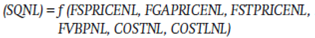
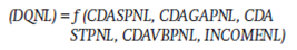
In the case of the Mexican strawberry supply, the variables analyzed were: strawberry production, frequent strawberry, Golden apple, saladette tomato and banana prices, and cost of production and labor (Equation 3). For demand they were: average Central de Abastos (market) price for strawberry, Golden apple, saladette tomato and banana, and income based on population and total GDP (Equation 4). Both data series were deflated, those of supply with the producer price index and those of demand with the consumer price index, published by (INEGI, 2016).
 (3)
(3)
Where:
SQNL = Mexico supply (production) quantity natural logarithm.
FSPRICENL = Mexico frequent strawberry price natural logarithm.
FGAPRICENL = Mexico frequent Golden apple price natural logarithm.
FSTPRICENL = Mexico frequent saladette tomato price natural logarithm.
FVBPNL = Mexico frequent Veracruz banana price natural logarithm.
COSTNL = Mexico cost of production natural logarithm.
COSTLNL = Mexico cost of labor natural logarithm.
 (4)
(4)
Where:
DQNL = Mexico demand quantity natural logarithm.
CDASPNL = Mexico Central de Abastos strawberry price natural logarithm.
CDAGAPNL = Mexico Central de Abastos Golden apple price natural logarithm.
CDASTPNL = Mexico Central de Abastos saladette tomato price.
CDAVBPNL = Mexico Central de Abastos Veracruz banana price natural logarithm.
INCOMENL = Mexico income natural logarithm.
Procedure to identify potentialities
With the support of data from official sources on areas planted and yields obtained in the last ten years, potential production volumes were determined by multiplying the maximum planted areas in the analyzed period by the highest yield obtained in this same time series (Table 1).
Table 1 Harvested strawberry area, yield and production in the period 2005 to 2014.
| Year | Harvested area (ha) | Yield (t∙ha -1 ) | Production (t) |
|---|---|---|---|
| 2005 | 2,664.13 | 26.16 | 69,698.97 |
| 2006 | 3,108.65 | 25.99 | 80,791.53 |
| 2007 | 3,139.75 | 28.38 | 89,095.30 |
| 2008 | 3,215.00 | 33.25 | 106,905.85 |
| 2009 | 3,561.00 | 32.23 | 114,784.00 |
| 2010 | 3,252.50 | 34.80 | 113,193.37 |
| 2011 | 3,351.00 | 34.07 | 114,170.72 |
| 2012 | 4,716.00 | 43.11 | 203,313.90 |
| 2013 | 4,482.50 | 45.72 | 204,937.15 |
| 2014 | 5,780.50 | 43.86 | 253,536.55 |
Source: Servicio de Información Agroalimentaria y Pesquera (SIAP, 2014).
Results and discussion
Characteristics of production processes
As a result of surveys applied at random, it was found that in Zamora, Michoacán, Mexico, producers have from 1 to 5 hectares devoted exclusively to strawberry cultivation, while intermediate-level producers have up to 30 ha, and large producers have an average of 100 ha. Regarding the technology used, the semi-technified, technified and to a lesser extent traditional farming operations predominate. The first two have irrigation drip tape systems. An estimated 70 % of the property is private and 30 % is ejidal.
Among the problems identified in the production processes are: low water quality, high well drilling costs, lack of technical advice during the production process, and the high cost of obtaining the strawberry plant, which is due to high royalty payments and labor costs.
Yield ranges between 30 and 70 t∙ha-1, of which only 40 % meets export quality and sells at $10.00 MXN per kg in the domestic market and from $10.00 to $40.00 MXN per kg in the international market.
The potential of Michoacán, Mexico, as a strawberry producer, in relation to the harvested area, is 5,896 ha, which is the maximum that has been planted in this state during the validated period (2005 to 2014). On the other hand, the yield potential, taking its maximum in the same period, corresponds to 45.72 t∙ha-1. Thus, considering both factors, maximum harvested area and maximum yield, a production capacity of 269,565.12 t was estimated for this state.
Production growth rate
Strawberry production during the validated period (2005 to 2014) had a growth rate of 7.1 %, distributed between its two components: area and yield (Table 2). An estimated 2.8 % was due to the increase in planted area and 4.3 % to yield increases. Based on the above, it can be inferred that the growth in strawberry production during the analyzed period is due, to a greater extent, to the technological change that has occurred in the study area, than to the increases in the planted area, thereby confirming the hypothesis stated earlier.
Table 2 Growth rate of strawberry cultivation during the period 2005 to 2014.
| Factor | Growth rate (%) | R 2 | Standard error | t value | Pr > ǀtǀ |
|---|---|---|---|---|---|
| Production | 7.1 | 0.8396 | 0.0086 | 8.25 | < 0.0001 |
| Area | 2.8 | 0.5414 | 0.0071 | 3.92 | 0.0018 |
| Yield | 4.3 | 0.9177 | 0.0036 | 12.05 | < 0.0001 |
Source: Author-made with data from the Servicio de Información Agroalimentaria y Pesquera (SIAP, 2014).
Forecasts
Forecasted quantities of strawberry exports from Mexico to the U.S. will retain their upward trend. Once the forecasts and the graph of the found and projected data are made, an ascending behavior is presented (Table 3). On the contrary, there is no indication that Mexico's strawberry exports will decline in the short or medium term.
Table 3 Mexican strawberry export forecasts for the period 2014 to 2020.
| Year | Forecasted strawberry exports (t) | R 2 | Standard error | t value | Pr > ǀtǀ |
|---|---|---|---|---|---|
| 2014 | 92,801 | 0.8552 | 333.45 | 11.40 | < 0.0001 |
| 2015 | 96,602 | ||||
| 2016 | 100,404 | ||||
| 2017 | 104,205 | ||||
| 2018 | 108,007 | ||||
| 2019 | 111,808 | ||||
| 2020 | 115,610 |
Source: Author-made with data from the model developed.
The statistical variables, object of analysis in the model developed in the Statistical Analysis System software (SAS, 2002), indicate that exports are 85 % explained by the model (Equation 5).
 (5)
(5)
The zero that precedes the variables T 2 and T 3 shows that there is no change in the growth trend of Mexico's strawberry exports.
Analysis of supply-demand in the United States
Economic theory establishes that the coefficient of a product’s price variable, when performing a supply equation, must be positive and in a demand equation it must be negative (Cramer, Jensen, & Douglas, 1988). For the other variables, such as the cost of production and labor, their supply coefficients must have a negative sign. In demand, the price of substitute products, as well as income, behave with a positive sign and complementary products with a negative sign. In this research there was correspondence with the signs according to economic theory (Table 4).
Table 4 Simple linear regression of strawberry supply and demand functions for the United States using logarithms.
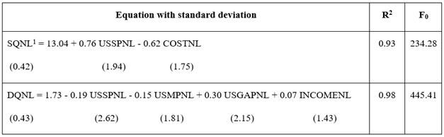
Source: Author-made based on the regression model.
1SQNL: U.S. supply (production) quantity natural logarithm; USSPNL: U.S. strawberry price natural logarithm; COSTNL: U.S. cost of production natural logarithm; DQNL: U.S. demand quantity natural logarithm; USSPNL: U.S. strawberry price natural logarithm; USMPNL: U.S. retail milk price natural logarithm; USGAPNL: U.S. Golden apple price natural logarithm; INCOMENL: U.S. income natural logarithm.
Note: The quantity supplied and demanded was in t and the prices in pesos per kilo. The income was in pesos per capita.
Regarding the statistical values, the quantity supplied is explained by the independent variables chosen in the supply model with 93 % R2 and an F-test value of 234.28, indicating that the U.S. strawberry price significantly affects the quantity supplied in that country. With 5 % of significance, all coefficients are statistically significant (Table 4).
Elasticities for the U.S. according to economic theory
The price elasticity of supply is inelastic, since in the case of a 1 % increase in the strawberry price, keeping everything else constant, the quantity supplied increases by 0.76 % (Table 4). This differs with the figure estimated by Carpio, Wohlgenant, and Safley (2008), who obtained a pre-harvest strawberry price elasticity of -1.30. The quantity supplied decreases by 0.62 % against the 1 % increase in the cost of production.
The statistical significance of the model was obtained by means of the coefficient of determination (R2), which indicates the goodness of fit of the estimated equations. The overall significance of the coefficients of each equation was observed with the F-test and the Student t distribution. The economic model was validated with the expected signs in the coefficients of each equation according to economic theory and the elasticities obtained in each equation (García-Mata, García-Salazar, & García-Sánchez, 2003).
The quantity demanded is explained by the independent variables chosen in the model, with R2 of 98 % and F of 445.41 in the regression performed, so the strawberry price in the U.S. significantly affects the quantity demanded. With 5 % of significance, all coefficients are statistically significant.
The price elasticity of strawberry demand in the U.S. is -0.19, which indicates that in the case of 1 % increases in the strawberry price, keeping everything else constant, the quantity demanded decreases by 0.19 %. Therefore, strawberry is an inelastic product. Richards and Patterson (1999) and Carter-Colin, Chalfant, Goodhue, and McKee (2005) estimated strawberry elasticity and found that it is very sensitive to price changes (-2.8 and from -1.2 to -2.7, respectively). These authors argue that these values varied over the course of the production season, being more elastic in May and June.
According to Cramer et al. (1988), the cross elasticity of strawberry demand with respect to the price of milk is -0.15 %, indicating that it is a complementary good. With a 1 % increase in the milk price, keeping everything else constant, the strawberry quantity demanded decreases by 0.15 %. On the other hand, this same parameter in strawberry with respect to the price of apple is 0.30, which shows that against 1 % increases in the price of 'Golden' apple the strawberry quantity demanded increases by 0.30 %. Therefore, apple is considered as a substitute good of strawberry.
The income elasticity of demand is 1.38 and, as in the previous case, suggests that strawberry demand increases by 1.38 % against a 1 % increase in income.
In this research, the price of strawberry to the US consumer has no effect on demand, unlike the shelf life of the strawberry, time spent obtaining the product and consumer preference, a fact that was also confirmed by Carpio et al. (2008).
Analysis of supply-demand in Mexico
The statistical parameters in the case of Mexico are: the quantity supplied is explained by the independent variables chosen in the supply model, with R2 of 64 % and F of 30.21 (obtained in the regression performed). It can be concluded that the strawberry price is not significant in the quantity supplied in Mexico, since it is governed by the price of the previous year (Table 5).
Table 5 Simple linear regression of strawberry supply and demand functions for Mexico using logarithms.
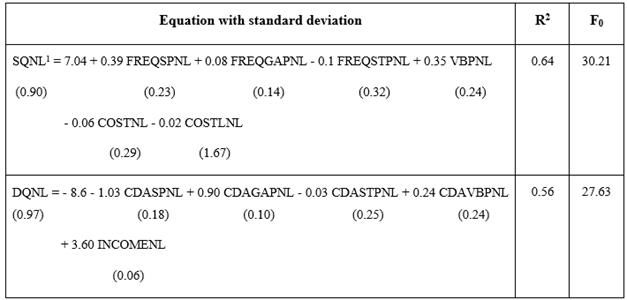
Source: Author-made based on the logarithmic regression model.
1SQNL: U.S. supply (production) quantity natural logarithm; FREQSPNL: Mexico frequent strawberry price natural logarithm; FREQGAPNL: Mexico frequent Golden apple price natural logarithm; FREQSTPNL: Mexico frequent saladette tomato price natural logarithm; VBPNL: Mexico frequent Veracruz banana price natural logarithm; COSTNL: Mexico cost of production natural logarithm; COSTLNL: Mexico cost of labor natural logarithm; DQNL: Mexico demand quantity natural logarithm; CDASPNL: Mexico Central de Abastos strawberry price natural logarithm; CDAGAPNL: Mexico Central de Abastos Golden apple price natural logarithm; CDASTPNL: Mexico Central de Abastos saladette tomato price natural logarithm; CDAVBPNL: Mexico Central de Abastos Veracruz banana price natural logarithm; INCOMENL: Mexico income natural logarithm.
Elasticities for Mexico
The price elasticity of the strawberry supply in Mexico is 0.39, which suggests that in the face of 1 % price changes, the quantity supplied changes by 0.39 % (Table 5). This coincides with the findings reported by Vázquez-Alvarado and Martínez-Damián (2011), since they mention that the supply and demand elasticity for Mexico’s main fruits is < 1.
The cross elasticity of the strawberry supply with respect to the price of apple is 0.08, banana 0.35 and saladette tomato -0.01, indicating that in the case of 1 % price changes, the supplied strawberry quantity increases by 0.08, 0.35 % and decreases by 0.01 %, respectively.
On the other hand, the elasticity of the cost of production and labor is -0.06 and 0.02, which shows that in the case of 1 % cost increases, the quantity supplied decreases by 0.06 and 0.02 %, respectively.
The variables selected for the Mexican demand model account for 56 % of the variation in quantity demanded. Both models, of supply and demand, in Mexico have a small R2, because of the low inclusion of complementary and substitute products.
The price elasticity of strawberry demand is -1.03, which makes it elastic; that is, in the case of 1 % price increases, the quantity demanded decreases by 1.03 %. This is in line with what has been established by Vázquez-Alvarado and Martínez-Damián (2011), who point out that the supply and demand elasticity of Mexico’s main agricultural products is < 1.
The cross elasticity with respect to the price of apple is 0.90, banana 0.24 and saladette tomato -0.03, meaning that in the case of a 1 % price change, the quantity of strawberry demanded increases by 0.90, 0.24 % and decreases 0.03 %, respectively. These values place the apple and the banana as substitute goods and the tomato as a complementary product of the strawberry.
The income elasticity of strawberry demand was 3.6, which indicates that in the case of a 1 % change in income, the quantity demanded increases by 3.6 %.
In Mexican strawberry production, labor is of great importance, since the product requires many day laborers, which has led to an improvement in the income level of working families and a greater rooting to their places of origin (Arana-Coronado & Trejo-Pech, 2014).
To determine whether the markets are in equilibrium, the supply and demand functions are equalized, taking into account the last price of the period studied (2014, Table 6).
Table 6 Equilibrium elements in the markets of the United States and Mexico.
| Element | U.S. | Mexico |
|---|---|---|
| Equilibrium price | $44.46 MXN per kg | $11.81 MXN per kg |
| Quantity supplied | QS1 = 1587.63 t | QS = 4105.16 t |
| Quantity demanded | QD = 1587.63 t | QD = 4105.16 t |
| Excess supply | 28.59 t | |
| Excess demand | 28.59 t |
Source: Author-made with data from models developed.
1QS: quantity supplied; QD: quantity demanded.
Production has two components: planted area and yield, both equal to 100 %. According to Zarazúa-Escobar, Almaguer-Vargas, and Márquez-Berber (2011), it is possible to separate them, obtain the proportion of each one and decide if the total growth in production is intensive, due to increases in area, or extensive, due to technological changes. In this work, it was observed that the increased production was because of yield, which leads to technological changes.
For Mexico, the outlook for strawberry exports is very encouraging, especially for those bound for the United States.
The equilibrium price between the two markets is $9.40 MXN per kg of strawberry, with excess supply and demand of 28.59 t. This validates the theory of Reed (2001), which mentions the existence of excess supply and demand, even though in this case it is a small quantity; in addition, it is interpreted as an existing potentiality. The above agrees with the views expressed by Hernández-Soto, Garza-Carranza, and Guzmán-Soria (2011), who specified that Mexico can still increase its export level, but not by 30 %, as found in this study, but 10 %.
Conclusions
Strawberry production during the validated period had a 7.1 % growth rate. Changes in planted area contributed 2.8 % and those of yield 4. 3 %. With this, it can be deduced that the increase in production was due more to technological change than to the increase in planted area.
According to the results of the cubic function, where the coefficients T2 and T3 are zero, it is concluded that the trend for Mexican strawberry exports, through the exponential model, is upward, both in the reported and projected data periods. There is no statistical evidence of a decrease or change in the short or medium term.
The price elasticity of the strawberry supply is inelastic in Mexico and the U.S. However, the price elasticity of demand is inelastic for the U.S. and elastic for Mexico. Therefore, it is concluded that there is still potential for increasing strawberry exports, strengthening the hypothesis that placing larger product quantities in the U.S. would have a favorable market outcome.

