


 texto en
  Inglés (pdf)
 Artículo en XML
 Referencias del artículo
 Enviar artículo por email
 Citado por SciELO
  Similares en
SciELO
Similares en
SciELO 
 Permalink
Introduction
Over the past decade, closed or semi-closed greenhouses have been successfully used in Europe and the United States because of the benefits in saving water and energy, and because of the increased efficiency of CO2 enrichment (Salazar-Moreno, Rojano-Aguilar, & López- Cruz, 2014), which is reflected in better yields and product quality. However, one of the problems associated with total or partial closure of the greenhouse is excess humidity, which can be avoided if the water vapor can be condensed without any dripping onto the crop (Baptista, Bailey, Randall, & Meneses, 1999). Most greenhouse structures do not achieve this aim; for this reason, semi-closed greenhouses have heat exchangers and gutters in the ceiling to carry out water vapor condensation.
In order to analyze the behavior of humidity in a greenhouse, it is necessary to simulate the water balance within it, for which there are several dynamic models that have been developed over the past 30 years. For example, Stanghellini (1987) analyzed the interrelationships between the microclimate and humidity surrounding the crop, and showed that the energy balance of a greenhouse crop provides a solid basis for quantifying the impact of microclimate on humidity and identifying limit values in climate management. The above-mentioned article reports the results of an experiment in which sub-models for the heat transfer of the foliage are defined; the sub-models were merged in an equation to obtain the temperature and transpiration of a greenhouse crop. The resulting estimates accurately reproduced the temperature and transpiration of a greenhouse tomato crop, as measured at time intervals of a few minutes (Stanghellini, 1987).
Jolliet and Bailey (1992)) took as a basis the Stanghellini (1987) model and measured the effect of some meteorological variables (air speed, vapor pressure deficit, solar radiation and CO2 concentration) on tomato transpiration, and studied climate control in a greenhouse by evaluating five transpiration models. For a young crop (leaf area index, LAI = 0.56) they found that an increase in solar radiation of 1 MJ∙m-2∙day-1 resulted in an increase in transpiration of 0.09 mm∙day-1, whereas an increase in vapor pressure deficit of 0.1 kPa increased transpiration by 0.013 mm∙day-1 and air speed of 1 m∙s-1 increased transpiration by 0.13 mm∙day-1. They also reported that for a more mature crop (LAI = 2.94), radiation had a slightly higher effect (an in crease of 1 MJ∙m-2∙day-1 caused an increase of 0.14 mm∙day-1), but the vapor pressure deficit was much higher (an increase of 0.1 kPa generated an increase of 0.24 mm∙day-1 in transpiration).
Jolliet and Bailey (1992) concluded that the transpiration rate increased linearly with solar radiation, vapor pressure deficit and air speed. Air temperature, CO2 concentration and heating pipe temperature had no significant effect on this rate.
Jolliet (1994), proposed the HORTITRANS model two years later to predict air humidity and crop transpiration as functions of outside weather conditions in order to develop optimal control strategies for humidity in greenhouses. This model includes the processes of transpiration, condensation, ventilation and humidification, and also allows the inside vapor pressure to be calculated as a function of outside conditions and greenhouse characteristics. Since the terms of the model are linear, it is possible to determine the amount of water and energy to be added to or extracted from the greenhouse air, in order to achieve humidity or transpiration set-points.
Stanghellini and de Jong (1995) emphasized the ventilation process in a greenhouse with natural ventilation and conducted an extensive analysis of the parameters related to it and the combined effect of temperature and wind.
Boulard and Wang (2000) presented a model to predict crop transpiration in a greenhouse. In it, the water vapor balance does not consider the condensation on the cover or on the heat exchangers in the ceiling, an important component when the greenhouse is closed. The estimates were better in summer than in spring, and comparisons with other transpiration models showed that considering outside conditions and not inside ones, as a boundary condition, involves deterioration in model performance. The authors attribute this to simplifications introduced during model derivation. Its performance was satisfactory when the greenhouse air was closely coupled to outdoor conditions.
Bontsema et al. (2007) conducted a review of the water balance in a greenhouse, including transpiration, condensation and ventilation flux equations, as well as the parameters involved; they also presented equations that consider the condensation on the ceiling and heat exchangers.
Since there have been few attempts to model the humidity within a semi-closed greenhouse, this paper uses as references the work conducted by Stanghellini and de Jong (1995), Bontsema et al. (2007), and Van Beveren, Bontsema, Van Straten, and Van Henten (2014), adapting some equations to develop a dynamic water balance model. To carry out the sensitivity analysis, the methodology presented by Saltelli, Chan, and Scott (2000) was used.
The aims of this study were: 1) to develop a dynamic model for the humidity behavior inside of a greenhouse when it is fully closed, 2) to develop a dynamic model for the humidity behavior inside of a greenhouse when there is natural ventilation and 3) to identify the most important parameters that influence the performance of both models by local sensitivity analysis and calibration.
Materials and methods
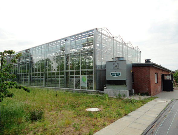
The study was conducted in a semi-closed greenhouse with tomato crop located at the Institute of Horticulture, Humboldt University of Berlin, Germany; this greenhouse has different characteristics than others, in that the energy storage tank is at the same level as the greenhouse, and not underground as is the case with most solar collectors.
The greenhouse is a Venlo type (Figure 1), measuring 24 x 12.8 x 6.7 m (length, width and height, respectively) and it is composed of four sections. The ground area is 307.2 m2, the volume 2,058.24 m3, the window area 51.2 m2, which represents 16.67 % of the ground area, and it has four ridges with a height of 1.4 m and a width of 3.2 m. The greenhouse is equipped with double glazing and a thermal screen, a cooling tower, a heat pump, and hydraulic switches, plus a 300 m3 capacity tank with water for energy storage, which is covered with insulation to prevent heat loss.
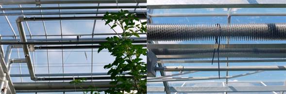
Plants function as a cooling surface. By transpiring, a plant is cooled and the water vapor rises towards the roof where the heat exchangers are located (in the form of corrugated pipes); there water circulates at dew point temperature, producing vapor condensation. Beneath the exchangers there are some gutters where the water from the condensation process is received and then conducted to a collection tank.
The condensation on the surface of the cover was not considered in this work since the heat exchangers placed under the ceiling capture most of the water (Figure 2).
The data used in this study were provided by staff at the Institute of Horticulture, Humboldt University of Berlin. The greenhouse has a weather station for measuring outside conditions, as well as a phytomonitoring system inside, where the main physiological variables are recorded every five minutes, such as transpiration, stomatal conductivity, photosynthesis, etc. Environmental variables such as temperature, relative humidity and CO2 concentration are recorded every 5 s with five sensors located at the ends and center of the greenhouse, and the measured values are averaged to obtain a datum every 30 s. The opening and closing of windows, as well as the maneuvering of the heating system, were obtained from greenhouse operation logbooks; for this, data from every 5 min, from January to September 2012, were used.
The model developed in this research is based on the one proposed by Bontsema et al. (2007), considering the specific case of a semi-closed greenhouse and the climatic conditions of the region.
Model 1: behavior of the air humidity in the completely-closed greenhouse.
In this dynamic model only transpiration and condensation processes were implemented.
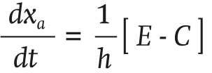
The differential equation describing the absolute humidity of the air xa (g∙m-3) inside the greenhouse is as follows:
 (1)
(1)
where E (g∙m-2∙s-1) is the plant transpiration, C (g∙m-2∙s-1) is the condensation on the heat exchangers and h (m) is the height of the greenhouse.
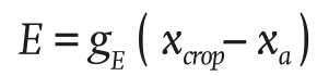
The water vapor flux due to plant transpiration E (g∙m-2∙s-1) is described in Equation 2:
 (2)
(2)
where gE (m∙s-1) is the transpiration conductance, xcrop (g∙m-3) is the water vapor concentration of the air at crop level and xa (g∙m-3) is the absolute humidity of the air inside the greenhouse.
The transpiration conductance gE is defined as follows:
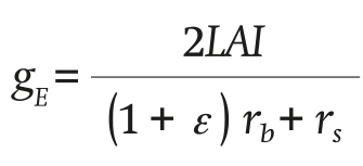 (3)
(3)
The ratio between latent heat and sensible heat content of saturated air ε (dimensionless) is determined in Equation 4:
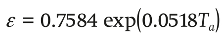 (4)
(4)
The leaf boundary layer resistance rb (s∙m-1) and stomatal resistance rs (s∙m-1) are described in Equations 5 and 6:
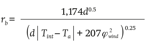 (5)
(5)
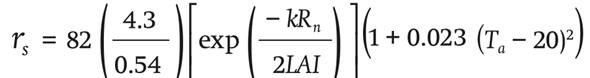 (6)
(6)
where Ta (°C) is the inside temperature, d(m)is the crop leaf length, Tint (°C) is the temperature of the heat exchanger,φwind (m∙s-1) is the wind speed inside the greenhouse and k (J∙u1) is the radiation extinction coefficient.
The net radiation absorbed by the canopy Rn (W∙m-2) is expressed as follows:
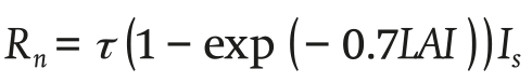 (7)
(7)
Where τ (dimensionless) is the transitivity coefficient of the cover, LAI is the leaf area index (dimensionless) and Is (W∙m-2) is the solar radiation outside.
The water vapor concentration of the air at crop level xcrop (g∙m-3) is given by the following Equation:
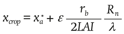 (8)
(8)
where λ (J∙g-1) is the latent heat of vaporization of water, and the saturated water vapor concentration (g∙m-3) is defined below:
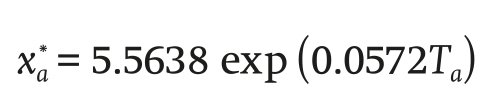 (9)
(9)
The absolute water vapor concentration of greenhouse air xa (g∙m-3) is a function of relative humidity (RH, %):
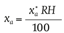 (10)
(10)
Finding the RH from Equation 10, and substituting with the expression
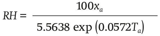 (11)
(11)
where xa (g∙m-3) is calculated through differential Equation 1.
Condensation of water vapor occurs on heat exchangers; it is collected in gutters and taken to a tank, so that evaporation can be disregarded.
The mass flow of water vapor C (g∙m-2∙s-1) in the greenhouse air due to condensation is:
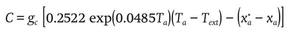 (12)
(12)
where Text (°C) is the outside air temperature and gc (m∙s-1) is the condensation conductance, and it is calculated the expression proposed by Van Beveren et al. (2014) :
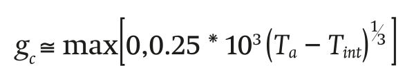 (13)
(13)
After the implementation of this model, the parameters were calibrated; this involved minimizing the sum of the squares of the errors between the humidity values predicted by the model and those measured, subject to the restrictions of the upper and lower limits of the parameters. With this procedure it was possible to find optimal values of the parameters that generated a better model fit.
Model 2: behavior of the air humidity in the semi-closed greenhouse with semi-closed windows.
In this model the transpiration, ventilation and condensation processes were considered. The first two processes were modeled in the same way as in the previous case.
The water vapor flux due to ventilation V was modelled with the Equation of Bontsema et al. (2007):
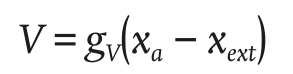 (14)
(14)
where gv (m∙s-1) is the condensation conductance and y xext (g∙m-3) is the absolute humidity of the outside air.
Following the model of Bontsema et al. (2007), the ventilation conductance is calculated as:
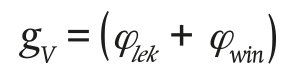 (15)
(15)
The infiltration φlek (m3∙s-1) is determined by the following Equation:
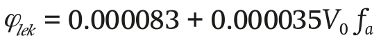 (16)
(16)
where V0 (m∙s-1) is the initial wind speed, and for the purposes of this model V0 = 1 and fa = 1 is a dimensionless infiltration factor.
The ventilation through the windows is given by:
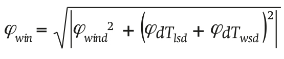 (17)
(17)
Where
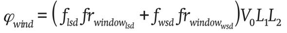 (18)
(18)
where L1
(m) is the length and L2
(m) the width of the
The leeward ventilation flsd (m3∙s-1) is determined in Equation 19:
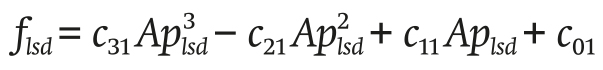 (19)
(19)
with c31 , c21 , c11 and c01 being empirical coefficients and Aplsd (dimensionless) is the number of leeward windows.
The windward ventilation fwsd (m3∙s-1) is:
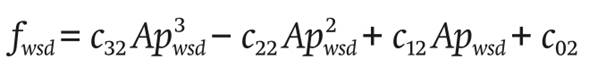 (20)
(20)
Likewise, c32 , c22 , c12 and c02 are empirical coefficients and Apwsd (dimensionless) is the number of windward windows.
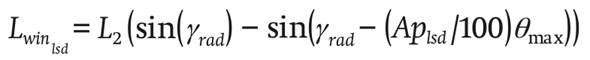
Leeward ventilation due to the temperature difference
 (21)
(21)
where a1
(dimensionless) is a transport coefficient, g (m∙s-1) the gravitational acceleration, Text
(°C) the outside temperature and
 (22)
(22)
γ (rad) is the slope of the roof and is given by Equation 23:
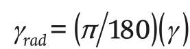 (23)
(23)
 (24)
(24)
Windward ventilation due to the temperature difference
 (25)
(25)
The length of the vertical opening of the window on the windward side
 (26)
(26)
The model was implemented in the MATLAB®/Simulink environment, which has a main program where the parameters, input variables and simulation options are defined, and a Simulink file where the model equations are implemented. The fourth-order Runge- Kutta method with ode45 integration variable step size, with a tolerance of 1 x 10⁻¹⁰, was used.
Results and discussion
Model 1: behavior of the air humidity in the closed greenhouse.
The initial values of the parameters used in this model were: 1) coefficient of the volume of air inside the greenhouse relative to the area thereof (H = 6.7 m) (data from the greenhouse under study), 2) leaf boundary layer resistance (rb = 200 s∙m-1) (Bontsema, et al. 2007), 3) radiation extinction coefficient (k = 0.8) (Carranza, Lanchero, Miranda, Salazar, & Chaves, 2008) and 4) light transmissivity (τ = 0.7) (Van Beveren et al., 2014). The results of the model’s implementation are shown in Figure 3, where overestimation and underestimation of the measured humidity can be seen. There is a poor fit of the measured to estimated values, so we proceeded to the calibration of the parameters to improve model performance.
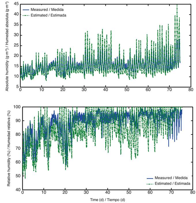
Figure 3 Absolute and relative humidity values, measured (blue) and estimated (green) with parameters reported in the literature (from February 15 to April 29, 2012)
Since the model has four parameters, the sensitivity analysis was omitted and we proceeded to calibrate the following: coefficient of the volume of air inside the greenhouse relative to the area thereof (H), leaf boundary layer resistance (rb ), radiation extinction coefficient (k) and light transmissivity (τ).
The calibration results are shown in Table 1, which has the initial and final fit measurements and the values of the parameters in both cases. It should be noted that we used different variation ranges, which were within the range reported in the literature. The best result obtained is reported in Table 1.
Table 1 Fit measures and optimal values of the parameters after calibration of model 1.
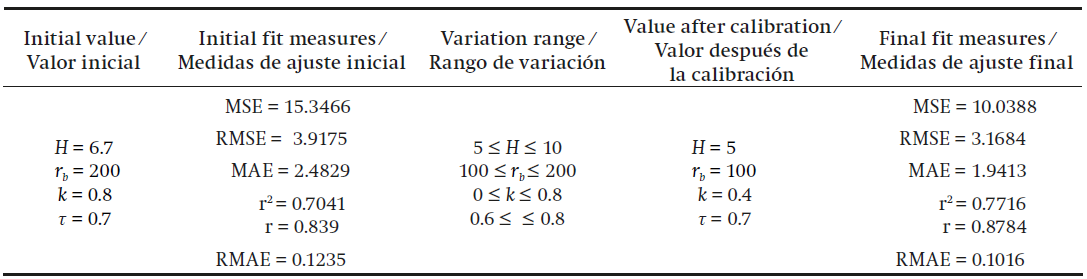
MSE = mean squared error, RMSE = root mean squared error, MAE = mean absolute error, r2 = coefficient of determination, r = correlation coefficient, RMAE = relative mean absolute error.
Once the optimal values were obtained, running the model resulted in a better fit, as seen in Figure 4.
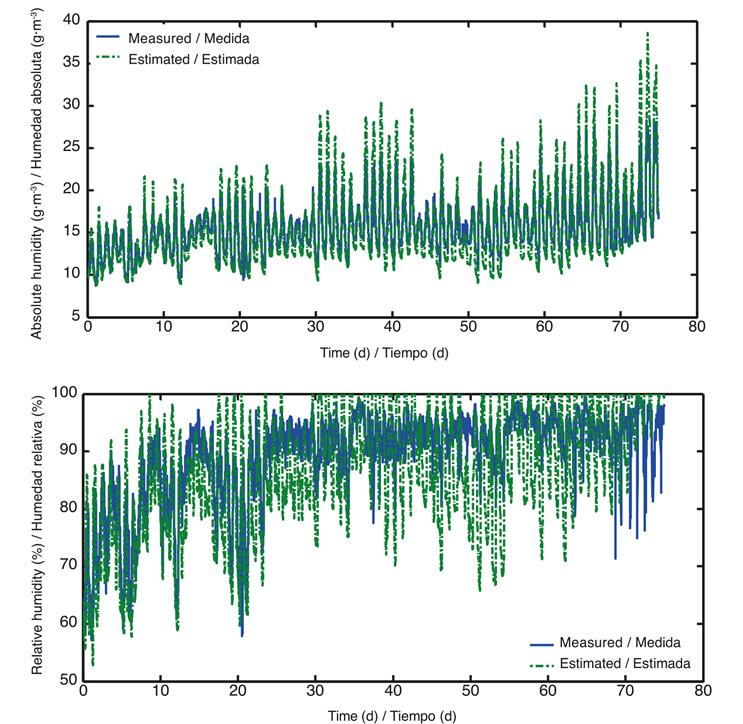
Figure 4 Absolute and relative humidity values, measured (blue) and estimated (green) with optimal parameters after calibration of the model.
There is no appreciable difference between Figure 3 and Figure 4 due to the amount of data considered in the simulation of model 1; therefore, a new run of the calibrated model was performed for two arbitrarily-chosen days, in order to observe the fit achieved (Figures 5).
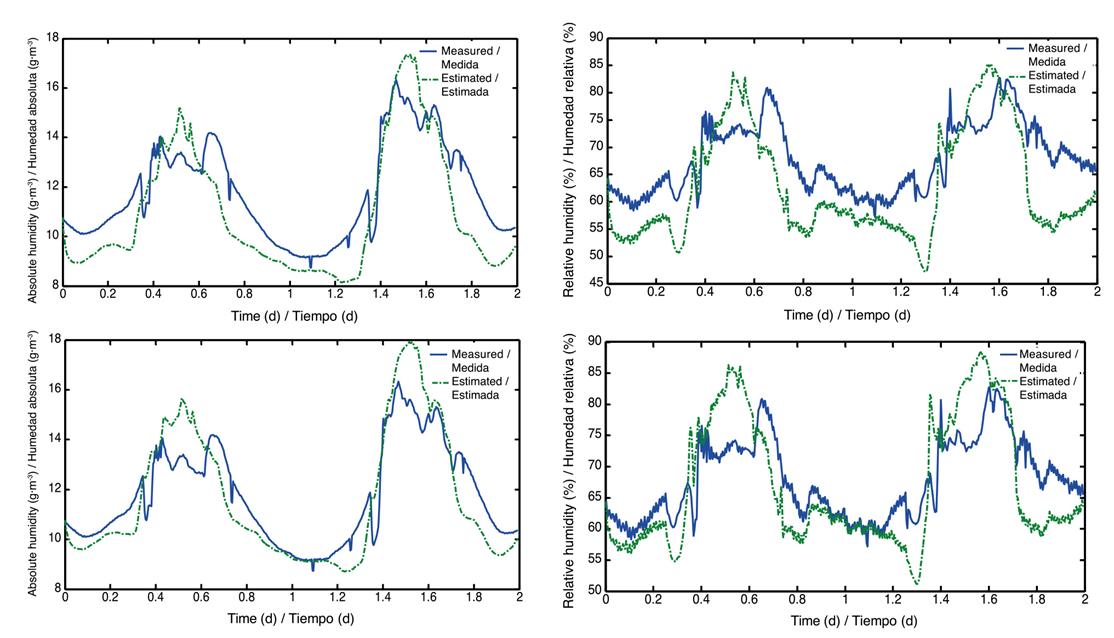
Figure 5 Values of absolute humidity (left) before and after calibration, and relative humidity (right) before and after calibration (February 15 and 16, 2012).
Considering the above results, it can be seen that the simulations of the completely closed greenhouse model have good approximation to measures at certain periods, whereas deviation is important for large humidity values.
Model 2: behavior of the air humidity in the semi-closed greenhouse when the windows are open.
For this model the processes of transpiration, ventilation and condensation were considered. To implement the third one, a sub-model of the specific ventilation was generated; this is joined by a subroutine to the main program of model 2.
The initial values of the parameters were: latent heat of vaporization of water (λ = 2,540 J∙g-1) (Van Beveren et al., 2014), radiation extinction coefficient (k = 0.8) (Carranza et al., 2008), window length (L1 = 3.2 m), number of windows (nv = 20), greenhouse ground área (As = 307.2 m2), window width (L2 = 0.8 m), leaf boundary layer resistance (rb = 200) (Bontsema, et al. 2007), roof slope (γ = 24.9 °) and light transmissivity (τ = 0.7) (Van Beveren et al., 2014). For the dimension values, the data from the greenhouse under study were used.
The simulation results and the parameters obtained from the literature are presented in Figure 6.
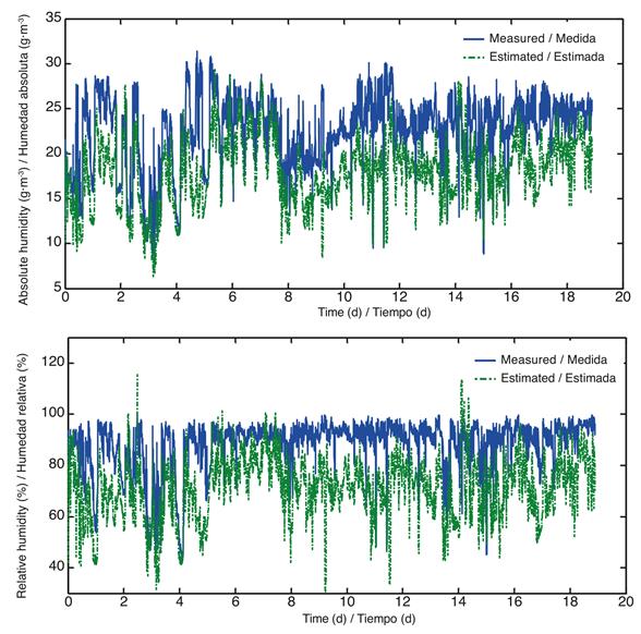
Figure 6 Values of absolute and relative humidity, measured (blue) and estimated (green) with parameters reported in the literature of model 2 (from March 9 to July 4, 2012).
It can be seen in Figure 6 that the model overestimates and underestimates the humidity inside the greenhouse. Since there is a greater number of parameters in this model, sensitivity analysis (Table 2), which aims to assess the relative importance of the parameters and constants on the evolution over time of the state variables and outputs (Saltelli et al., 2000), was performed; for this reason the dimensions of the greenhouse were included.
Table 2 Values of the sensitivity indices for parameters λ, k, L 1, n v, A s, L 2, r b , γ and τ .
| Parameter | Sensitivity indices | ||
|---|---|---|---|
| Relative sensitivity index of absolute humidity | Relative sensitivity index of relative humidity | Absolute sensitivity index of absolute humidity | |
| λ | 1.3721 x 10¹¹ | 1.3721 x 10¹¹ | 1.1112 x 10⁹ |
| k | 5.2802 x 10⁴ | 5.2802 x 10⁴ | 1.3437 x 10⁸ |
| L 1 | 3.0172 x 10⁴ | 3.0172 x 10⁴ | 1.8261 x 10⁵ |
| nv | 3.0172 x 10⁴ | 3.0172 x 10⁴ | 2.9218 x 10⁴ |
| A s | 3.0172 x 10⁴ | 3.0172 x 10⁴ | 1.9022 x 10³ |
| L 2 | 1.6123 x 10⁴ | 1.6123 x 10⁴ | 3.8178 x 10⁵ |
| rb | 1.3671 x 10⁴ | 1.3671 x 10⁴ | 2.4836 x 10³ |
| γ | 486.0123 | 486.0123 | 404.1606 |
| τ | 6.2290 | 6.2290 | 1.6065 x 10⁴ |
The calibration results of the model are displayed in Table 3, for which the most sensitive parameters (λ, k, L1 , nv , As , L2 and rb ) were used.
Using the already calibrated values in Table 3, model 2 was implemented, resulting in a better performance of the estimation of the model with respect to the measures (Figure 7).
Table 3 Fit measures and optimal values of the parameters after calibration of model 2.
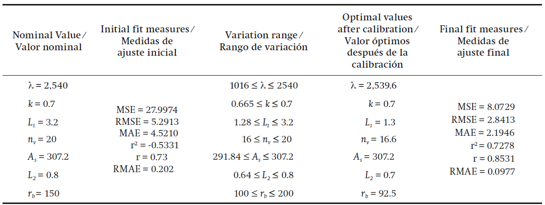
MSE = mean squared error, RMSE = root mean squared error, MAE = mean absolute error, r2 = coefficient of determination, r = correlation coefficient, RMAE = relative mean absolute error.
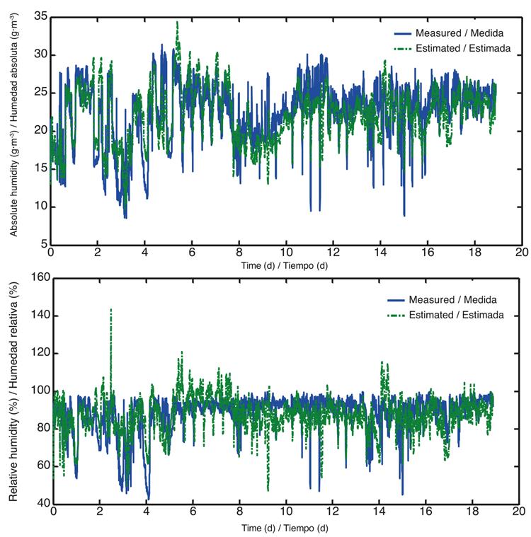
Figure 7 Absolute and relative humidity values, measured (blue) and estimated (green) with optimal parameters after calibration of model 2.
In order to observe in greater detail the fit that was achieved after calibration, the model was implemented for seven days (Figures 8).
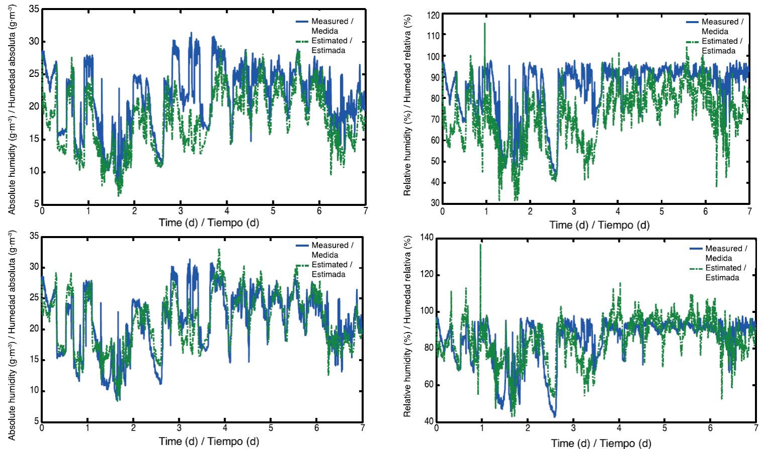
Conclusions
In the first dynamic model, calibration of the height of the greenhouse (H), which measured 6.7 m up to the ridge, and decreased to 5 m, was performed. This means that the greenhouse is oversized, with a height greater than needed to perform its functions.
The aerodynamic resistance (rb) reported in the literatura was 200 s∙m-1 (used as the upper limit in the calibration) and after calibration an rb = 100 s∙m-1 was obtained, meaning that the lower the boundary layer resistance, the higher the transpiration rate. The radiation extinction coefficient (k) decreased by half after calibration; that is, the amount of radiation captured by the canopy up until reaching the lower foliage layers was lower, perhaps because in a semi-closed greenhouse there are major obstacles for the radiation to pass, such as sensors and heat exchangers placed among the foliage. Finally, the transmissivity coefficient of the cover τ = 0.7 (reported for a glass greenhouse by Van Beveren et al., 2014) did not present variation after calibration, which is congruent, since the conditions of the Netherlands and Germany are not very different in terms of geographical location, andgreenhouse type and management. After calibration of model 1, it was possible to reduce the MAE from 2.4829 to 1.9413, and r increased from 0.839 to 0.8784.
In the second model, the calibration result showed that the latent heat of vaporization of water (λ) and the radiation extinction coefficient (k) remained constant. This coefficient is related to the inclination angle of the leaves and provides information on how efficient the plant is in intercepting solar radiation. In this sense, model 2 is more efficient, perhaps due to the movement of the leaves that allows radiation penetration. The length, width and number of windows decreased after calibration, which means that the ventilation area can be reduced. Also, rb decreased from 150 to 92.5, lower than the value found for model 1, which is reasonable since ventilation decreases aerodynamic resistance.
After calibration of model 2, it was possible to reduce the MAE from 4.52 to 2.19 and r increased from 0.73 to 0.8531.
Both models were able to detect the parameters and constants involved in the water balance.

