


 nueva página del texto (beta)
 Inglés (pdf)
 Artículo en XML
 Referencias del artículo
 Enviar artículo por email
 Citado por SciELO
  Similares en
SciELO
Similares en
SciELO 
 Permalink
INTRODUCTION
Historically, humanity has faced the complication of obtaining water because it is a necessary and indispensable resource in our daily activities. In many locations, surface water for human consumption has diminished over the last several decades leading to a necessary increase in groundwater extraction, particularly in many arid and semi-arid regions. For this reason, many semiarid regions have experienced a considerable reduction of groundwater storage as pumping has greatly exceeded natural recharge. Subsequently, researchers in these critical regions are focusing on studies aimed at understanding recharge processes and determining effective ways in which recharge can be enhanced naturally (Carrillo-Rivera, 2000, Carrera- Hernández et al., 2016, Manna et al., 2017, Müller et al., 2016; Scanlon, et al., 2010; Sharda, et al., 2006). Groundwater recharge (GWR) refers to the entry of meteoric water across the water table after first entering the soil zone. Recharge crossing the water table potentially enhances aquifer storage. GWR can occur in two ways, by a downward movement due to the gravity forces in the form of runoff and infiltration or by horizontal movement, which generally occurs as lateral contributions of groundwater flow from adjacent aquifers. Factors such as rate and direction of GWR depend on the hydraulic parameters of the geologic layers that make up the soil profile and aquifer systems in question (Balek, 1988). Groundwater recharge is one of the most important parameters in quantifying sustainability of aquifer systems. Several different methods have been employed to evaluate the quantity of recharge entering aquifer systems. These include physical and hydrogeochemical methods and numerical models (Scanlon et al. 2006, Simmers 1998, Scanlon et al. 2002). Other study factors such as: slope, depth to groundwater, infiltration rate, are used to determine the areas most suitable for groundwater recharge (Ghayoumian et al. 2007) or in the application of geographic information systems (SIG) and numerical modeling (Chenini et al. 2010). These factors are also used in the study of the temporal and spatial variation of recharge, along with the application of natural or artificial tracers (Hernández-Marín et al. 2018, Allison et al. 1994, Sophocleous 1991, Wang et al. 2008, Qin et al. 2011). It is worth mentioning that some techniques do not attempt to quantify an actual GWR rate, but rather estimate potential GWR, a term that refers to the water that infiltrates but does not instantaneously contribute to the aquifer storage, but rather where subsurface drainage actively participates so that the net storage change is not easily quantifiable. For example, in areas with a thick unsaturated zone, the direct influence of the rainfall on the water table and then on GWR varies both temporally and spatially depending on the hydrogeological conditions of the subsoil, precipitation pattern (e.g. intensity and duration) and evapotranspiration, as well as the geomorphological characteristics of the surface (Rushton, 1988, Scanlon et al., 2002). Taking these aspects into consideration, it becomes important to quantify the drainage in a rigorous manner to minimize the error in the quantification of an actual recharge rate that affects overall aquifer storage (Cuthbert, 2010).
In recent years, analytical techniques have been proposed for the evaluation of GWR. Many of these approaches assume that temporary changes in the groundwater level are controlled by two main factors: the balance of recharge and net drainage of groundwater (Crosbie, et al., 2005; Cuthbert, 2010; Jie, et al., 2011). These two factors can be applied to GWR when the aquifer systems are separated from the surface by a thick vadose zone. In this way, the potential recharge of aquifers under known climatic conditions depends mainly on the infiltration from surface water bodies and the lateral contributions.
The aim of this research is to evaluate the potential GWR by applying an analytical adjustment of the Water Table Fluctuation (WTF) technique, in combination with the Boussinesq equation for the quantification of drainage. This methodology is applied to the aquifer of the Aguascalientes Valley, where the territory is classified as semi-arid (POEA, 2013) and 94% of water use originates from underground sources (CONAGUA and SEMARNAT, 2016). The WTF method is based on two intrinsic factors of the aquifer: (1) variations of the static water levels and (2) specific yield. The Boussinesq equation is related to hydraulic conductivity and aquifer thickness (or transmissivity). A further goal is to create a recharge map containing isovalues over the study area and the variations in the recharge isovalues will be discussed in the context of the overall hydrogeology of the region. This analysis will raise awareness about the sustainable management of the local aquifer, as well as to help in decision-making of actions such as the establishment of waste disposal areas, or the delimiting of areas vulnerable to groundwater pollution and to better understand their possible occurrence.
CHARACTERISTICS OF THE STUDY AREA
The study area corresponds to the valley of Aguascalientes in the state with the same name, occupying a strip having a North-South orientation and extending a length of approximately 80 km and a width of 25 km as shown in Figure 1. This zone is in a tectonic graben as described by Aranda-Gómez (1989).
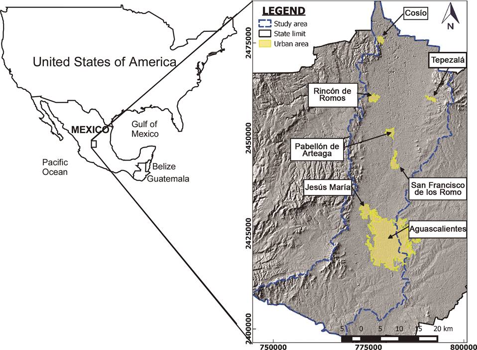
The San Pedro River represents the main hydrographic feature of the Valley and flows from north to south almost through the center of the valley. The main land uses in the study region include agriculture with intensive irrigation and livestock (63%), natural pasture (16%), shrubs (15%), oak forest (3.9%), mesquites (0.2%), with the remaining 1.9% corresponding to urban areas, where more than 85% of the population of the state resides (CONABIO et al., 2008, INEGI, 2018). It is important to mention that of the 50 thousand hectares dedicated to the agricultural activities within the valley, almost the entire area is irrigated with groundwater, although there is an important potential for the reuse of groundwater from irrigation, (CONAGUA, 2005; Pacheco-Martínez et al., 2013). In terms of climate, 68% of the territory of Aguascalientes is semi-arid with an average maximum temperature of 25 °C, and an annual average rainfall of 526 mm and annual average potential evaporation of 2,200 mm. The rainy season occurs mainly during summer, with only occasional rainfall during the other seasons of the year (INEGI, 1993).
Geomorphologically, the study area is relatively flat with small hills distributed within the area and increasing slopes toward the mountains. The valley is located between the Tepezalá mountains of to the east and the Sierra Fría mountains in the west. The average altitude of the Aguascalientes Valley is 1,900 m. The valley includes two important physiographic provinces. The Mesa Central is in the east, while the Sierra Madre Occidental is to the west and consists of valleys and elongated mountain ranges oriented mainly NW-SE and NE-SW (CONAGUA, 2018). According to UNAM-UAQ (unpublished data, 2002) a predominance of alluvial and fluvial deposits occurs within the valley with the topmost sedimentary sequence composed primarily of detrital rocks derived from unconsolidated alluvial materials and classified as clays, silts, sands and gravels according to their grain size. The general stratigraphic sequence was determined through vertical electric soundings (SEVs) that were performed throughout the study area (Zermeño-Villalobos, 2016). Beneath the detrital rocks it was determined that the unconsolidated deposits exhibit a variable thickness from a few meters in the periphery of the valley, to up to 380 meters in the center (Hernández-Marín et al. 2018). Approximately 200-300 meters of compacted lithified sediments (conglomerates and sandstones) and fractured igneous rocks (rhyolites and ignimbrites) occur below the fluvio-alluvial refill that occupies the center of the valley. The compacted conglomerates outcrop mostly in the west, while igneous rocks can be observed in the east, conforming to the orientation of the mountain ranges. An analysis of the lithology of the unconsolidated central sediments was evaluated based on the SEV results and the lithological records of deep well logs, which suggests a stratigraphic configuration of coarse sediments such as gravel and sand, with smaller portions of clay and silt. Groundwater is determined to flow from north to south according to water level observations from measured wells. The chief aquifer of the Aguascalientes valley is considered unconfined (DOF, 2012), but with a thick vadose zone. As expressed by some local drilling engineers (Fuentes-López, expert in geophysics and geology, personal communication, 2018), currently no uprising of water levels in wells occurs during drilling, despite the presence of a thick vadose zone. Therefore, the local aquifer is considered as free or unconfined because this type of aquifers is defined by its response to groundwater pressure, regardless of the thickness of the vadose zone.
METHODOLOGY
Conceptualization and analysis of the WTF technique and the quantification of drainage
According to Vélez-Otálvaro (2004) the methods to determine the GWR can be classified into five categories: direct measurements, water balance, chemical tracers, Darcy-Law approximations, and empirical methods. This author also states that some of the most reliable methods for estimating the recharge of semi-arid zones such as the Aguascalientes valley are chemical tracers, direct measurements and water balance. In this research the water balance method is used to quantify recharge and specifically invokes the method of variations of groundwater, defined as Water Table Fluctuation or WTF. This method has been used in several research investigations. Healy and Cook (2002), for example, presented an excellent review of theory and its applications. Cuthbert (2010) performed an analysis that includes underground drainage to minimize the error in the recharge estimate by developing an expression for the drainage component, which is a function of the hydraulic gradient and transmissivity and therefore hydraulic conductivity and saturated thickness. In general, the WTF technique is applicable to several hydrologic scenarios, including ones in which the water table is deep and / or where groundwater levels can vary smoothly, if the hydrogeological properties of the aquifer are relatively well known.
The expression used in the method assumes that temporal water-level changes of an aquifer are controlled by the recharge balance R (mm/year) and the net drainage of groundwater D (mm/year) at a given observation point for a certain period of time, t. The recharge can be calculated as:
Where S y represents the specific yield, ∂h/∂t is the temporal variation of the water table in the study area, and D is the drainage.
The WTF method frequently ignores factors such as trapped air or barometric fluctuations that may affect the water level (Healy and Cook, 2002). In addition, the water that infiltrates and moves through the unsaturated zone can vary significantly in time and quantity, depending on certain conditions such as evapotranspiration, porosity, hydraulic conductivity, specific yield, and depth. The main limitations of the WTF technique are the difficulties of defining and estimating the specific yield as well as the quantification of drainage in areas with thick unsaturated zones, since in shallow water tables, the error in drainage may be minimal because the water level may increase significantly during a rainfall period. Therefore, in areas with a considerably deep water table, it is important to rigorously estimate the drainage to minimize the error in the quantification of the recharge, as suggested by Cuthbert, (2010). This author also establishes the equation for the drainage calculation considering the case of an ideal homogeneous horizontal aquifer limited at one end with x = 0, conceptually representing a boundary without flow (e.g. the mountains along the basin perimeter), and at the other end with x = L where a river exists and exhibits a constant head boundary condition, as shown in Figure 2. This idealized scenario is a typical conceptual representation of many aquifer systems.
The calculation of the drainage is based on the one-dimensional Boussinesq equation of the groundwater flow for an aquifer that receives homogeneous recharge and that follows a sinusoidal pattern. The applicable equation is the following:
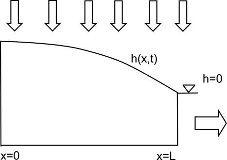
Figure 2 Idealized conceptual section of an aquifer that receives recharge with sinusoidal variation of the water level h (x, t) (Cuthbert, 2010).
Where T is the transmissivity (m²/d) and
By combining equations 1 and 2, the recharge and drainage can be calculated for a period of time as:
Specific Yield (S y ) estimation
The specific yield S y is a fundamental parameter in the WTF method and can be defined as the volume of water released per unit area of the unconfined aquifer when the water table decreases by one unit of height. However, this definition is only valid under conditions of equilibrium and small-scale experiments. Currently, there are several methods to measure S y , such as laboratory, fieldwork, empirical, etc. However, they all have a degree of associated uncertainty. Commonly, S y is assumed to be a constant value (Healy and Cook, 2002, Tritscher et al., 2000), although this parameter varies depending on the different intrinsic conditions of the aquifer such as the local water flow, the depth of the phreatic level and the heterogeneity of the soil (Fetter, 2001). Thus, its variability depends on the factors that are considered for its calculation and the means in which they are obtained (Childs, 1960). The specific yield is inherently treated as a storage term independent of time in the WTF method, which in theory explains the instantaneous release of stored water.
APPLICATION OF THE METHOD
Estimation and distribution of specific yield S y
The distribution of the specific yield throughout the study zone was mapped based on the results of two previous investigations, (UNAM-UAQ unpublished data, 2002; CONAGUA 2015).
In the first report, a numerical groundwater model was developed using the Visual-Modflow package program, in which a map of the variation of S y was developed through model calibration, which yielded a S y isocurve map for year 1996. The researchers used a total of 160 wells during their modeling analysis. In the second report, the results of 13 pumping tests ranging from hours to days were performed in the north and center of the Aguascalientes Valley. Time-drawdown curves were developed from the pumping tests and compared with the theoretical curves developed by Boulton (1963), Neuman and Witherspoon (1972) and Moench (1996) for the calculation of the specific yield at each pumping test location. Linear interpolation was then used to create a map of the variations of S y in the area where the pumping tests were performed. The S y maps from both investigations were combined algebraically using the multilevel B-spline interpolation method to create a new map of the variation of the specific yield in the study area. The new map is shown in Figure 3.

Figure 3 Distribution of the specific yield in the study area. This map combines the results from UNAM-UAQ (unpublished data, 2002) and CONAGUA (2015) using the interpolation Multilevel B-Splines method.
Evaluation of groundwater levels
Groundwater levels were obtained by analyzing data provided by government agencies such as PROACTIVA medio Ambiente CAASA, which is the company commissioned for the distribution of water in the municipality of Aguascalientes, and the CONAGUA. Both agencies provided the static water levels of wells measured throughout the Valley during the period 1968-2015. This investigation focuses only on the period between 1985 and 2015. Figure 4 shows a map with the location of the wells with the provided data, the measurements in the wells are mostly annual and sometimes monthly.
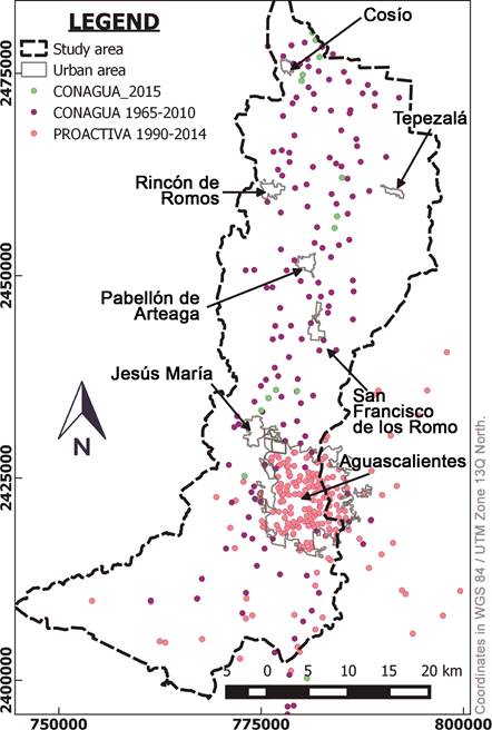
Figure 4 Location of wells used in this study and provided by CONAGUA and PROACTIVA Medio Ambiente CAASA.
Unfortunately, as in many cases, not all the wells have complete data that could be used for direct application of the method, thus, a classification of the wells was performed in order to discard those without sufficient information. To determine which and how many wells would be included in the study, we first considered those active during 2015, recalling that this is the most recent year of the analysis period. The availability of regular measurement records was also considered. In some cases, the missing data was completed by applying one of four statistical methods according to the amount of missing data and the location of the well in the valley. The methods applied were linear regression, neighborhood averages, average ratios and the correlation method. As a final analysis, 145 wells were used for the application of the WTF technique.
Estimation of underground drainage
To estimate the underground drainage, the methodology described by Cuthbert (2010) was considered. As mentioned earlier, this author proposed a conceptual model with the section of a free aquifer of length x = L. In the study area, this model is represented by a section of the basin of the Aguascalientes valley, where the San Pedro River would form a constant hydraulic head boundary, while the model periphery represents a no-flow condition at x = 0 as shown in Figure 5 (see also Figure 2 and Eq. 3).

Figure 5 All sections (represented as horizontal lines) on the Aguascalientes valley were used to estimate the drainage, with x = 0 representing the no-flow boundary, and x = L representing a constant-head boundary, which coincides with the location of the San Pedro River through the center of the valley.
The values of transmissivity were taken from reports of various agencies of both public and private sectors (Table 1). Similarly, as was done for creating a map of S y , the B-Spline Multilevel technique was used as an interpolation method to obtain the distribution of the transmissivity distribution in the study area as shown in Figure 6.
Table 1 Transmissivity values taken from various agencies of the public and private sectors (CONAGUA, 2015). Coordinates in WGS 84 / UTM Zone 13Q North.
| Well ID |
UTM Coordinate | T (m2/day) |
Well ID |
UTM Coordinate | T (m2/day) |
Well ID |
UTM Coordinate | T (m2/day) |
Well ID |
UTM Coordinate | T (m2/day) |
||||
|---|---|---|---|---|---|---|---|---|---|---|---|---|---|---|---|
| X | Y | X | Y | X | Y | X | Y | ||||||||
| 68-22 | 775938 | 2416730 | 846.72 | 42-79 | 778242 | 2441802 | 648 | 27 | 788605 | 2425861 | 13.0464 | III | 785023 | 2418770 | 409.536 |
| 51-50 | 782121 | 2434346 | 388.8 | 42-33 | 780569 | 2444860 | 864 | 34 | 783284 | 2422929 | 655.776 | X | 790796 | 2452293 | 607.392 |
| 33-43 | 780214 | 2452735 | 1123.2 | 33-52 | 784818 | 2455822 | 138.24 | 41 | 782917 | 2422196 | 402.624 | VIII | 794399 | 2449891 | 9.504 |
| 23-4 | 777303 | 2461804 | 518.4 | 43-4 | 798648 | 2445439 | 250.56 | 44 | 782137 | 2422104 | 538.272 | VII | 799734 | 2448679 | 72.4896 |
| 24-57 | 786328 | 2461753 | 544.32 | 23-3 | 775953 | 2462251 | 181.44 | 53 | 783513 | 2421050 | 384.48 | VI | 772512 | 2461130 | 55.0368 |
| 3-10 | 777821 | 2484558 | 362.88 | 24-6 | 781780 | 2470351 | 475.2 | 56 | 782871 | 2419905 | 686.016 | IV | 778544 | 2465290 | 1161.993 |
| 78-6 | 780934 | 2406973 | 95.04 | 15-2 | 780668 | 2480729 | 250.56 | 58 | 784385 | 2420180 | 113.184 | V | 783632 | 2465257 | 209.952 |
| 68-16 | 774098 | 2417086 | 146.88 | 41 | 787028 | 2475627 | 19.872 | 64 | 781765 | 2416606 | 26.0928 | 88 | 779641 | 2476307 | 11.7504 |
| 79-1 | 799641 | 2412077 | 1468.8 | 1 | 779000 | 2485523 | 551.23 | 66 | 785165 | 2419492 | 13.1328 | 7A | 786555 | 2474032 | 55.1232 |
| 60-26 | 779474 | 2425622 | 129.6 | 19 | 778799 | 2482188 | 436.32 | 69 | 786770 | 2418943 | 12.8736 | 90 | 779302 | 2468233 | 13.824 |
| 50-64 | 775976 | 2433108 | 26.784 | 3 | 781994 | 2430787 | 51.235 | 98 | 789155 | 2415186 | 2.68704 | 68 | 777563 | 2447623 | 58.4928 |
| 51-87 | 790663 | 2435136 | 23.328 | 9 | 785164 | 2429507 | 8.0697 | I | 783485 | 2418911 | 1099.958 | 172 | 772481 | 2431870 | 7.56 |
| PAB-4 | 790683 | 2438531 | 49.248 | 21 | 782129 | 2424253 | 328.32 | II | 784144 | 2417735 | 244.512 | 178 | 780264 | 2399489 | 5.14944 |

Figure 6 Distribution of transmissivity. Map resulting from the Multilevel B-Splines interpolation and the data of Table 1.
RESULTS
The GWR was calculated for each of the 145 wells using Eq. 3 along with the isocurves from Figures 3 and 6. The calculated GWR and the parameters used in the computation are compiled in Table 2 (which only shows the results of 30 wells for brevity). This table also includes some of the annual data over the span of the 30-year analysis.
Table 2 Representative sample of results of the application of the WTF method (Δh*) and the analytical solution of the Boussinesq equation (D*) for the estimation of GWR (R*). The differences in the value of the column of Sy and T are determined by the location of the well on the maps of specific yield and transmissivity, respectively.
| Well ID |
UTM Coordinates |
(m) |
x* (m) |
L* (m) |
T* (m2/d) |
D* (mm/d) |
S y * |
Δh* (mm) |
R* (mm/year) |
|
|---|---|---|---|---|---|---|---|---|---|---|
| X | Y | |||||||||
| 1 | 778394.6 | 2484628 | 0.020 | 4108.600 | 9267.440 | 423.360 | 0.087 | 0.004 | 36926.781 | 5.134 |
| 4 | 781311.2 | 2480026 | 0.015 | 4108.600 | 9267.440 | 259.200 | 0.042 | 0.004 | 53880.000 | 7.406 |
| 6 | 780709.7 | 2476737 | 0.010 | 4108.600 | 9267.440 | 86.400 | 0.010 | 0.004 | 57869.300 | 7.918 |
| 7 | 783861.7 | 2477367 | 0.004 | 4108.600 | 9267.440 | 181.440 | 0.008 | 0.004 | 85882.023 | 11.745 |
| 10 | 778877.9 | 2471298 | 0.004 | 5647.180 | 14086.210 | 293.760 | 0.005 | 0.080 | 57729.936 | 153.951 |
| 11 | 786033.2 | 2470462 | 0.004 | 12846.190 | 14411.690 | 259.200 | 0.018 | 0.004 | 51989.000 | 7.124 |
| 12 | 781580.1 | 2470578 | 0.004 | 8457.590 | 13485.980 | 432.000 | 0.012 | 0.004 | 60167.400 | 8.235 |
| 13 | 788169.5 | 2473568 | 0.021 | 5373.620 | 7070.390 | 98.323 | 0.070 | 0.004 | 64326.668 | 8.862 |
| 14 | 785940.1 | 2470072 | 0.037 | 12696.830 | 14518.230 | 267.494 | 0.145 | 0.004 | 6655.400 | 1.054 |
| 15 | 778958.6 | 2476200 | 0.011 | 2176.640 | 9161.830 | 42.336 | 0.004 | 0.004 | 46484.005 | 6.357 |
| 17 | 778468.7 | 2465203 | 0.001 | 5791.200 | 14414.310 | 1140.480 | 0.007 | 0.100 | 49921.400 | 166.411 |
| 18 | 781394.1 | 2463445 | 0.002 | 7230.370 | 12755.150 | 437.184 | 0.006 | 0.200 | 55283.600 | 368.563 |
| 19 | 784890.3 | 2467963 | 0.009 | 12411.420 | 14881.270 | 3162.240 | 0.321 | 0.004 | 52230.800 | 7.460 |
| 20 | 779191.5 | 2460838 | 0.002 | 5933.510 | 13432.770 | 451.872 | 0.006 | 0.100 | 52855.500 | 176.191 |
| 21 | 785664.4 | 2461996 | 0.007 | 11204.060 | 12330.950 | 535.680 | 0.096 | 0.082 | 56919.500 | 155.676 |
| 22 | 784988.9 | 2462107 | 0.006 | 10587.270 | 12199.260 | 453.600 | 0.056 | 0.200 | 48847.704 | 325.707 |
| 23 | 780607.9 | 2461276 | 0.004 | 6786.290 | 12907.140 | 449.280 | 0.010 | 0.082 | 65161.700 | 178.119 |
| 25 | 777425.6 | 2457806 | 0.000 | 4378.570 | 13380.330 | 419.040 | 0.000 | 0.082 | 44765.546 | 122.359 |
| 27 | 777473.5 | 2442462 | 0.006 | 7211.950 | 13387.010 | 599.616 | 0.019 | 0.082 | 44147.392 | 120.689 |
| 28 | 780722.9 | 2458545 | 0.004 | 8737.350 | 14505.950 | 428.544 | 0.008 | 0.100 | 65455.900 | 218.195 |
| 30 | 783625.3 | 2452290 | 0.001 | 13941.470 | 16109.780 | 518.400 | 0.004 | 0.082 | 58538.500 | 160.009 |
GWR shown in Table 2 was converted into a digital map for further analysis. The results reveal the regions with the highest and lowest estimated GWR within the study area. The greatest recharge is located mainly in the northern and central parts of the valley, where a maximum recharge of 525.67 mm/year is estimated. Conversely, at the north and south boundaries of the study site, as well as in the metropolitan area of the city of Aguascalientes, the lowest values of GWR are estimated to be on the order of 0.086 mm/year. Figure 7 shows the calculated distribution of the recharge for the study area.

DISCUSSION
The results from Figure 7 clearly show that the center and north portions of the valley have the largest rates of GWR. These areas of high recharge can be attributed in part to the dominant type of soil, which corresponds to course-grained alluvial deposits with relatively high values of specific yield and hydraulic conductivity (0.010 to 0.30 and 0.2 to 20 m/d respectively). Furthermore, as a consequence of the predominance of this type of soil, the estimated drainage increases in the vicinity of the San Pedro River, which is likely enhanced by extensive agricultural practices in this area due to the high return volume of irrigation water to the subsoil. Conversely, the regions with the lowest estimated rates of GWR, located at the north and south boundaries of the valley, as well as in the metropolitan area of the city of Aguascalientes, is attributed to the large discharge of groundwater that lowers water levels and consequently thickens the vadose zone and results in reduced levels of estimated recharge. Also, possibly contributing to the reduced estimates of recharge is, the presence of sandstones and conglomerates exhibiting a low specific yield and small hydraulic head variations. Interestingly, these low recharge areas are where the highest calculated contributions by drainage occur. Clearly, the high drainage does not appear to make a significant difference in the general estimation of recharge.
When comparing the recharge estimated in this study with that estimated by UNAM- UAQ (unpublished data, 2002) using natural tracers (O-18 and Deuterium) the zones with the largest potential for recharge coincide with the results estimated in this investigation. Furthermore, they also determine that the zone with the lowest potential for recharge is within the city of Aguascalientes, which also coincides with the results presented here.
On the other hand, an estimation of natural recharge reported by CONAGUA (2018) takes into account a water balance with four factors: underground horizontal flow input based on the static level and Darcy's law (83.1×10⁶ m³), horizontal flow outputs with an estimated volume of 2.4×10⁶ m³, pumping of 427.4×10⁶ m³ and storage change, taking into account the configuration of the evolution of the static level registered during the period 2000-2014, with an annual average of -180.2×10⁶ m³, the natural recharge estimated by CONAGUA is 249.6×10⁶ m³, but if only the vertical recharge is taken into account CONAGUA recharge is 166.5×10⁶ m³, which is 0.9% less than the total recharge estimated in this investigation (168×106 m³). It should be noted that in the technique described here, does not consider the horizontal recharge. Despite the different methods used in the calculation of the vertical recharge, the results are almost equal, these comparisons indicate that the technique proposed in this work is applicable to the Aguascalientes valley, although it may be necessary to apply new methodologies or to include new factors in the future to reduce uncertainly in estimated recharge. Some of the factors to consider may be water bodies, effects of anisotropy, and climate data for long-term periods.
CONCLUSIONS
This investigation presents a methodology for the estimation of groundwater recharge (GWR) by employing an analytical solution of Boussinesq for unconfined flow into the Water Table Fluctuation (WTF) method. The study area encompasses the semi-arid valley of Aguascalientes, in central Mexico. This rectangular north-south trending valley represents a tectonic graben that is about 80 km in length and 25 km in width. The estimated GWR is variable throughout the valley with an estimated maximum annual value of 526.26 mm and a minimum annual rate of 0.86 mm. The areas with the greatest estimated recharge are located at the northern and central parts of the valley and is attributed to agricultural practices and coarser-grained soils in these areas. Conversely, the lowest estimated recharge occurs along the north and south boundaries of the study area and within the city of Aguascalientes. These low values are attributed to heavy pumping, which lowers the water level and increases the thickness of the vadose zone as well as to lithologies having a low specific yield. The results present similarity in volume and space, with previous studies.

