


 nueva página del texto (beta)
 Inglés (pdf)
 Artículo en XML
 Referencias del artículo
 Enviar artículo por email
 Citado por SciELO
  Similares en
SciELO
Similares en
SciELO 
 Permalink
Introduction
A large portion of the Mexican territory is privileged with the presence of volcanic and tectonic activity, which has led to the formation of convective hydrothermal systems (Arango-Galván et al., 2015). An effective installed capacity of ~920.4 MWe is currently produced from high-temperature geothermal resources, which contribute with nearly 2.1% of the electricity annual production (Bertani, 2016; SENER, 2017). High-temperature geothermal fields of Cerro Prieto in Baja California, Los Azufres in Michoacán, Los Humeros in Puebla, Las Tres Vírgenes in Baja California, and the Domo of San Pedro in Nayarit are currently exploited for electricity production with an effective installed capacity of 570 MWe, 225 MWe, 80.4 MWe, 10 MWe, and 35 MWe, respectively (SENER, 2017). The Cerritos Colorados geothermal field in Jalisco, with an estimated potential of 75 MWe, has also been identified as a promissory zone (Flores-Armenta, 2013; Pandarinath and Domínguez, 2015). An updating map of geothermal resources of Mexico that includes the geothermal fields under exploitation, and the most promissory zones under exploration are shown in Figure 1a.
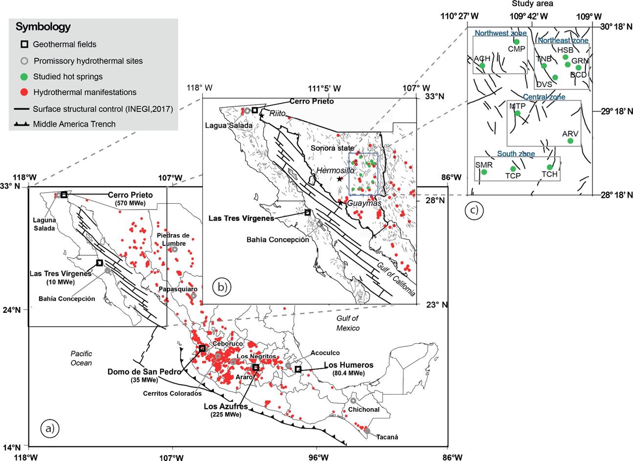
Figure 1 a) General map showing the current geothermal fields under exploitation and promissory hydrothermal sites of Mexico; b) Projected simplified map of Sonora state; c) Study area and location of the sampled thermal springs in four zones: Huasabas (HSB), Bacadehuachi (BCD), Cumpas (CMP), Granados (GRN), Arivechi (ARV), San Marcial (SMR), Tecoripa (TCP), Tonichi (TCH), Divisaderos (DVS), Tonibabi (TNB), Matape (MTP), and Aconchi (ACH).
Low-to-medium temperature geothermal systems, t<200 °C (also referred as low-to-medium enthalpy systems) in several regions of Mexico have not been exploited yet for electricity generation, although a total installed capacity of ~156 MWth has been quantified (Prol-Ledesma and Canet, 2004; Gutiérrez-Negrín et al., 2015; Morales-Arredondo et al., 2016). The primary use of these resources has been in balneology, notwithstanding the large amount of resources available for direct uses, which is estimated in 40,589 MWth (Romo-Jones et al., 2017). A complete inventory of these geothermal resources was reported by Iglesias (2003).
From this inventory, the presence of promissory hydrothermal systems in the northwestern part of Mexico has been highlighted by Hiriart et al. (2011). These geothermal systems have been delimited from geological, geophysical, and geochemical prospecting studies. Prol-Ledesma and Juárez (1986) quantified, in a preliminary geophysical study carried out in the same region of Mexico, heat fluxes of 100 mW/m2, which were based on reservoir temperatures inferred from SiO2 geothermometry. Based on direct measurements of heat flux performed in exploration wells, Prol-Ledesma (1991) measured more accurate heat fluxes up to 191 mW/m2 for the same regions.
Other promissory zones with a geothermal potential have also been identified in Sonora (Mexico) by Verdugo-Mariscal (1983), Prol-Ledesma (1991), Torres et al. (1993), Barragán et al. (2001), Iglesias et al. (2011), and Almirudis et al. (2015): see Figure 1b. Verdugo-Mariscal (1983) reported the presence of geothermal zones that coincide with NE-SW morphological structures possibly related with the spreading centres of the Gulf of California. This author suggested the existence of a hydrothermal system characterized by two types of SO4-Cl waters:
(i) medium-enthalpy fluids with estimated geothermometric temperatures up to 189±21 °C, which interact with rocks of lithological units from the Paleozoic to the Cretaceous and Tertiary volcanics; and (ii) low-to-medium enthalpy fluids with estimated geothermometric temperatures up to 143±5 °C, which are interacting with rocks from the continental Tertiary, which were sealed by younger clay rocks.
Prol-Ledesma (1991) carried out a study for evaluating thermalized water aquifers of Guaymas (Sonora). Using the chemical composition of water samples collected from wells, the fluids were classified as HCO3 and Na-Cl waters with a variable concentration of SO4. By applying some solute geothermometers, deep equilibrium temperatures up to 115 °C were predicted, which were in good agreement with direct measurements of geothermal gradients.
Torres et al. (1993) reported the existence of thermal springs of Na-HCO3 waters, which are associated with NNW-SSE regional structures in eastern Sonora. Using a comprehensive database, Iglesias et al. (2011) reported the existence up to 154 hydrothermal springs located in Sonora with surface temperatures ranging from 28 to 88 °C.
Barragan et al. (2001) reported a geochemical survey for studying Na-Cl fluids with temperatures up to 192 °C, emerging from artesian and deep wells drilled in the Riito zone (located in the eastern side of the Colorado river in the NW part of Sonora). These fluids were typified as high-saline sedimentary waters, which are isotopically similar to those waters found in the Mexicali valley, and which are poorly affected by meteoric waters. This hydrothermal system was related to adjacent fault systems of Cerro Prieto.
Finally, Almirudis et al. (2015) carried out an exploration campaign in the central and eastern zones of Sonora, and briefly reported the probable origin of the geothermal fluids found in some hot springs. Reservoir temperatures and water-rock interaction processes were roughly analysed for developing a preliminary geochemical model. A detailed study on these zones was proposed for a better characterization of these low-to-medium geothermal resources, from where the present study is derived.
All these previous geochemical surveys, along with the Quaternary and recent volcanism (Paz-Moreno et al., 2003; García-Abdeslem and Calmus, 2015), the relative geographical nearness to Cerro Prieto and Las Tres Vírgenes geothermal fields, and the active tectonics of the Gulf of California, seem to identify the Sonora State as a region of Mexico with a promissory geothermal potential (1b). The geological, geophysical and geochemical features enable the hydrothermal systems of Sonora to be studied in more detail for a better evaluation of their geothermal reserves.
The goal of the present study is to report a more comprehensive geochemical model for the evaluation of the low-to-medium temperature geothermal systems located in the east-central part of Sonora. The new geochemical model is based on a fluid geochemistry database of shallow hot springs (containing the composition of major and trace elements, as well as the isotopic signatures of oxygen and deuterium), including the pseudo-equilibrium state conditions found in the system as a result of the fluid-rock interaction that governed the formation of these hydrothermal zones.
The study also aims to describe the major hydrochemistry signatures of hot springs in terms of fluid classification, the geochemometric determination of the most probable reservoir temperatures, the geothermal fluid sources, and the local fluid mixing processes. Meteorological data available for these geothermal sites were also analysed to evaluate the possible influence of meteoric water recharge, and the variability of the most common climatic parameters, including the surface and ambient temperatures.
Geological setting
The geology of southwestern North America was dominated by a subduction period since at least the mid-Cretaceous until the middle Miocene: from southern Mexico up to Canada, the Farallon-Kula oceanic plates were subducted to the East beneath the North American continental plate (Atwater, 1989). As a result of this subduction process, between 90 and 40 Ma, a large volume of magmatic intrusive and volcanic rocks were emplaced in the Sonora State. The plutonic rocks produced from this intrusive event are known as the Sonora Laramide Batholith (Damon et al., 1983), whereas the volcanic rocks from the same geological event are referred as the Tarahumara Formation (Wilson and Rocha, 1949; McDowell et al., 2001) or the Lower Volcanic Complex (McDowell and Keizer, 1977; Ferrari et al., 2005, 2007). These rocks are widely distributed in the eastern and central Sonora State.
Towards 50 and 42 Ma, a reorientation of the Pacific plates occurred together with a decrease in the convergence velocity between the Farallon-Kula and North American plates (Stock and Molnar, 1988). This reorientation triggered a progressive change in the magmatism of Mexico and southwestern United States, inducing the emplacement of enormous volumes of ignimbrites during the late Eocene-Oligocene. The resulting rocks constitute the Sierra Madre Occidental (SMO), which are known as the Upper Volcanic Complex, and are recognized as one of the largest ignimbrite provinces in the world (McDowell and Keizer, 1977; Cochemé, 1985; Ferrari et al., 2007). During Oligocene-Miocene, the North American plate and the Eastern Pacific ridge came into contact, giving end to the subduction period. A sinking of the lithosphere was produced and a thermal flux along Sonora and California resulted in low angle fault movements (Stock and Molnar, 1988). During the middle Cenozoic a distension period of large scale was produced in southern Sonora, with a northwest-southeast orientation (Gans, 1997). The volcanic plateau was fragmented to the east and west of the SMO, resulting the current morphology of the Basin and Range (Stewart, 1978), which is also present in the Sonora and Chihuahua States in Mexico. This morphology of parallel mountains and valleys, delimited by normal faults, has different degrees of sedimentary accumulation in their basins. The most ancient sediments, locally known as the Baucarit Formation (King, 1939; Cochemé et al., 1988), present basalt intercalations dated at 23-19 Ma (Demant et al., 1989; Paz-Moreno, 1993; McDowell et al., 1997).
A peralkaline acidic ignimbritic volcanism in Central Sonora, dated at 12.5 Ma, emphasizes an important change in the source of magmas. It corresponds to the latest stage of continental extension prior to the marine invasion and the development of spreading centers in the Gulf of California (Vidal-Solano et al., 2005). This ignimbritic episode is related to a large-scale extension and lithosphere thinning that induced the formation of an intra-continental rift. This ‘proto-Gulf’ occurred before trans-tensional deformation and spreading operated in the Gulf of California as a consequence of new Pacific-North America plate boundary motions (Oskin and Stock, 2003).
As result of the establishment of a transitional regime in the Gulf of California, between a divergent limit in the central and southern areas and a transforming limit to the north, the present tectonic configuration was established with the formation of the first pull-apart basins approximately 4 Ma (Martín-Barajas, 2000). Nowadays the limit between the North American and the Pacific plates is governed by the rift system of the Gulf of California-San Andreas fault.
Quaternary volcanism of the Sonora state is roughly represented by different rock outcroppings (Paz-Moreno, 1993; Lynch et al., 1993). One of these outcrops is the Moctezuma basaltic field, which is placed within the northeast zone of the geothermal study area of the present research. This volcanic field is characterized by the transition from fissure type tholeiitic basaltic volcanism to alkaline scoria cones, with intermittent activity between 1.7 and 0.5 Ma (Paz-Moreno et al., 2003). More recently, a basalt flow from this Quaternary volcanism, that impounds a Bison-bearing fossil deposit at Térapa, Sonora, was dated to 440-130 ka using whole rock 40Ar/39Ar (Bright et al., 2010). A simplified geological map of the study area is available in the map collection of the Servicio Geológico Mexicano (Geological Survey of Mexico https://www.sgm.gob.mx/GeoInfoMexGobMx/). A detailed map of the geological setting of the northeast zone of Sonora is schematically shown in Figure 2.

Promissory geothermal zones of the Sonora State
The study area containing the promissory geothermal zones is located approximately 50 km in straight line to the east of Hermosillo city (the capital of the Sonora State), in the SMO mountain portion of east-central Sonora (see Figures 1b and 1c). Schematic geological cross sections of the study area are shown in Figure 3. In this area, twelve geothermal localities were identified with a hydrothermal activity in association with hot spring waters (see Figure 1c). These localities have been geochemically grouped in four major hydrothermal zones: the Northwest (NW) zone which is characterized by the shallow hot springs from Aconchi (ACH) and Cumpas (CMP); the Northeast (NE) zone which is characterized by the shallow hot springs from Tonibabi (TNB), Huasabas (HSB), Divisaderos (DVS), Granados (GRN), and Bacadehuachi (BCD); the Central (C) zone which is characterized by the shallow hot springs from Matape (MTP) and Arivechi (ARV); and the South zone (S) which is characterized by the shallow hot springs from San Marcial (SMR), Tecoripa (TCP) and Tonichi (TCH).
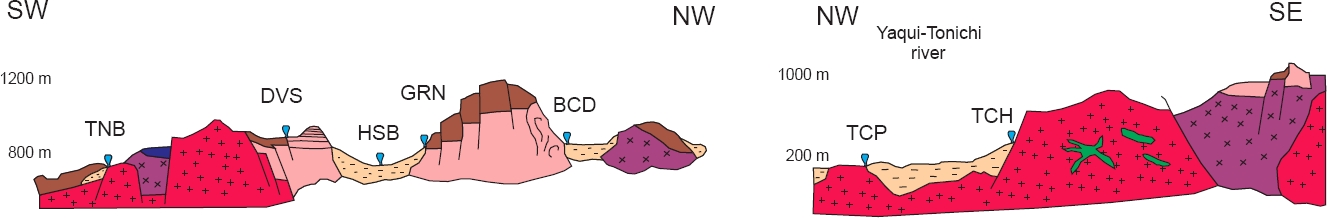
Figure 3 Schematic geological cross sections of the northeastern and southern zones of the study area (same legend as in Figure 2).
The NE zone contains a Lower Cretaceous detritus-carbonated sedimentary sequence (Lawton et al., 2004), which is cut by Upper Cretaceous volcanic rocks, and correlated with the Tarahumara Formation. Both sedimentary and volcanic sequences are intruded by a series of plutonic rocks (Roldán-Quintana, 1994; Almirudis, 2010) (Figure 2). Tertiary rocks correlated with the Upper Volcanic Complex cover the whole series of rocks (Cochemé, 1985). The basins are filled with alluvium and sediments from the Baucarit Formation, and, particularly the Moctezuma valley, with basalts of the Quaternary Moctezuma volcanic field. The NW, C, and S zones present similar lithologies to those in the NE zone, although lacking Quaternary volcanism. Furthermore, some of their outcrops correspond to ancient rocks composed mainly by carbonated sedimentary rocks (limestones and dolomites) and sandstones (see Figures 2 and 3).
Climatological data
The climate of the study area can be categorized as semiarid. The highest annual rainfall generally occurs on July, and it ranges from 114 to 175 mm, whereas for the dry season, which generally occurs on May, the rainfall is lower than 3 mm. The lowest and highest annual evaporation values are 84 mm and 331 mm, respectively. The air temperature over this area varies from a maximum value of 42 °C in the summer time (on June) up to a minimum temperature of 2 °C in winter (mainly on January). Table 1 summarizes the average annual climatological measurements collected from six meteorological stations located in the study area (BCD, HSB, DVS, MTP, ARV, and TCH). These data were compiled from the Eric III Climatological Database v.1.1 (IMTA, 2013).
Table 1 Annual climatological measurements collected from the Eric III National Database v1.1 (IMTA, 2003).
| Station name |
Longitude W |
Latitude N |
Altitude (m a.s.l.) |
Average record time (days) |
Min Temp Intervala (oC) |
Max Temp Intervala (oC) |
Rainfall Intervala (mm) |
Evaporation Intervala (mm) |
|---|---|---|---|---|---|---|---|---|
| BCD | -109.283° | 29.767° | 706 | 1129±67 | 2±3 (Jan) 21±2 (Jul) 12±5 (Oct) |
21±4 (Jan) 38±3 (Jun) 31±5 (Oct) |
6±12 (May) 114±52 (Jul) 27±32 (Oct) |
84±21 (Jan) 317±68 (Jul) 153±35 (Oct) |
| HSB | -109.300° | 29.903° | 570 | 198±21 | 4±3 (Jan) 22±2 (Jul) 13±4 (Oct) |
22±4 (Jan) 41±4 (Jun) 324 (Oct) |
4±7 (May) 132±61 (Aug) 41±40 (Oct) |
102±32 (Jan) 331±33 (Jun) 147±8 (Oct) |
| TNB | -109.567° | 28.583° | 217 | 1538±58 | 8±3 (Jan) 24±2 (Jul) 18±4 (Oct) |
27±5 (Jan) 42±4 (Jun) 364 (Oct) |
5±10 (Apr) 175±79 (Jul) 31±38 (Oct) |
N.R. N.R. N.R. |
| DVS | -109.033° | 29.600° | 680 | 279±35 | 5±3 (Jan) 22±3 (Jul) 15±4 (Oct) |
21±3 (Jan) 38±3 (Jun) 315 (Oct) |
5±8 (May) 146±58 (Jul) 30±33 (Oct) |
N.R. N.R. N.R. |
| MTP | -109.500° | 29.100° | 718 | 453±33 | 8±3 (Jan) 19±5 (Jul) 15±4 (Oct) |
23±5 (Jan) 37±3 (Jun) 31±5 (Oct) |
3±6 (May) 168±80 (Jul) 23±26 (Oct) |
112±24 (Jan) 308±54 (Jun) 158±44 (Oct) |
| ARV | -109.183° | 28.933° | 566 | 853±45 | 8±3 (Jan) 19±5 (Jul) 13±4 (Oct) |
24±4 (Jan) 40±3 (Jun) 34±5 (Oct) |
5±10 (May) 160±61 (Jul) 26±33 (Oct) |
151±0. (Sep) 293±0. (Jul) 158±0. (Oct) |
aThe parameter measurement interval considers records from the lowest to the highest values. The climatological data of 2003 are reported as a reference for the time of the sample collection campaign.
Methodology
The methodology used in this prospection study is based on a novel and fundamental diagram of water-rock interaction (WRI) and chemical partitioning processes associated with geothermal environments, which was originally described by Libbey and Williams-Jones (2016). A simplified diagram showing some tracing paths of these processes (applied to the present study) is shown in Figure 4. For describing the fluid fractionation, the WRI paths used are shown with double dot connection lines, and frameworks without filled patterns (‘A-A1-A2-A3-A4-A5-A7’).
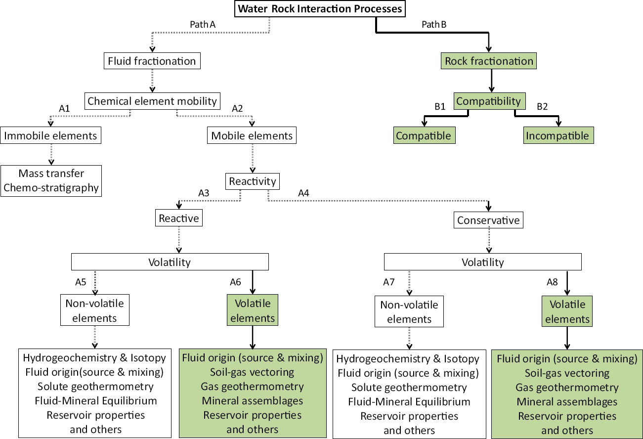
Figure 4 Schematic diagram showing the water-rock interaction (WRI) and chemical partitioning processes associated with geothermal environments (modified after Libbey and Williams-Jones, 2016).
Chemical and isotopic signatures were defined as key geochemical parameters for the fluid fractionation study. The chemical mobility of major and trace elements was therefore studied by using chemical analyses of hot spring waters from the four hydrothermal zones of Sonora (NW, NE, C, and S). Reactive (Na, K, Ca, Mg, SO4, SiO2, F, among others) and conservative (Cl, Br, the ‘Rare Alkalis’: Li, Rb, Cs, among other) elements were used for finding out some geochemical signatures of the fluids produced in the reservoir (Giggenbach, 1991). The use of bulk-rock components as geochemical tracers of fluid paths contributes to a comprehensive understanding of element mobility and reactivity in these geothermal systems (Libbey and Williams-Jones, 2016).
Fluid sampling and chemical analyses
For the fieldwork, a geochemometric programme was used for the collection and analysis of representative water samples from the identified hydrothermal zones. Major physicochemical parameters were in situ measured. A HACH portable multimeter (equipped with temperature and electrical conductivity sensors), and a HANNA portable potentiometer were used for measuring temperature, and pH of the hot spring waters. All the pH measurements were recorded with the temperature compensation option after calibration with standardized buffer solutions of pH 4.0, 7.0 and 10.0. Measurement errors of pH (accuracy and precision) were typically better than ±0.1 pH units (±1.4%); whereas for the temperature and electrical conductivity measurements, the errors were better than ±1.1 °C (±2.6%) and ± 33 µS/cm (±3.0%), respectively. Ten replicates of all these measurements were systematically recorded in the hot spring discharges. Total alkalinity (HCO3 - and CO3 2-) was determined in situ, by triplicate, after sampling by using a titration method with a micro-burette according to the standardized analytical methodology proposed by Nicholson (1993). Gas samples were not collected because steam vents or fumaroles were not observed in the study area. Small gas bubbling sites were intermittently found in a few zones with very low discharge flow rates, which made difficult their collection.
Polyethylene bottles of 500, 100, and 50 mL volume (previously washed with HCl and rinsed three times with deionized water) were used for collecting water samples to be used in the chemical analysis of major (anions and cations, and other compounds) and trace (metals) elements, as well as for the isotopic analyses (18O/16O, and D/H). For the analysis of anions, hot spring waters were collected without adding acid, whereas for the determination of cations, the water samples were preserved by adding ultrapure HNO3 to pH < 2. All these water samples were previously filtered through a 0.2 μm membrane filter.
Chemical analyses (major and trace elements) were carried out at Actlabs Laboratories (Canada), whereas the isotopic analyses were conducted at the Isotope Laboratory of the University of Arizona (USA). Major cations and trace elements were determined by Inductively Coupled Plasma-Mass Spectrometry and Inductively Coupled Plasma-Optical Emission Spectrometry, whereas the anions were analysed by ion chromatography. The stable isotopes of 18O/16O and D/H were analysed by gas source Isotope-Ratio Mass Spectrometry. Table 2 summarizes the precision and accuracy errors (in %) reported for the chemical analyses, including the limits of detection (LOD’s), for each one of the elements. Accuracy was evaluated by analysing water certified standards as external testers. Ionic charge balances were calculated among the major cations (Li+, Na+, K+, Ca2+, and Mg2+) and anions (F−, Cl−, NO3 -, SO4 2-, PO4 3-, and HCO3 -) for checking the quality of the chemical analyses of hot spring waters.
Table 2 Precision, accuracy and detection limits for the elemental chemical analyses.
| Chemical Elements |
Precision (%) |
Accuracy (%) |
LOD | Chemical Elements |
Precision (%) |
Accuracy (%) |
LOD |
|---|---|---|---|---|---|---|---|
| Major elements | Trace elements | ||||||
| Cations | Ru | ND | ND | 0.01 | |||
| Li+ | 9 | 5.9 | 0.001 | Pd | ND | ND | 0.01 |
| Na+ | 5 | 9.5 | 0.005 | Ag | ND | ND | 0.2 |
| K+ | 1 | 10 | 0.03 | Cd | 8.3 | -2.1 | 0.01 |
| Mg2+ | 2.2 | 1.6 | 0.002 | In | ND | ND | 0.001 |
| Ca2+ | 2.3 | 5.9 | 0.7 | Sn | ND | ND | 0.1 |
| Anions | Sb | 5 | -2.4 | 0.01 | |||
| F- | 8.3 | -1.6 | 0.01 | Te | ND | ND | 0.1 |
| Cl- | 1.3 | 0.4 | 0.03 | I | ND | ND | 1 |
| NO2 - | 2.6 | 3.6 | 0.01 | Cs | 0.6 | 15 | 0.001 |
| NO3 - | 0.9 | -0.7 | 0.01 | Ba | 0.8 | 5 | 0.1 |
| SO4 2- | 1 | 1.6 | 0.03 | Hf | ND | ND | 0.001 |
| PO4 3- | 2.1 | 5.5 | 0.02 | Ta | ND | ND | 0.001 |
| HCO3 - | 3 | 3 | 1 | W | ND | ND | 0.02 |
| Re | ND | ND | 0.001 | ||||
| Trace elements | Os | ND | ND | 0.002 | |||
| Be | ND | ND | 0.0001 | Pt | ND | ND | 0.3 |
| Al | 0.5 | 10.3 | 2 | Hg | ND | ND | 0.2 |
| Si | 1.6 | 10.5 | 200 | Tl | 2.6 | -12.7 | 0.001 |
| Sc | ND | ND | 1 | Pb | ND | -11.5 | 0.01 |
| Ti | 4.6 | -14.3 | 0.1 | Bi | ND | -12.1 | 0.3 |
| V | 10 | 4.5 | 0.1 | Th | 5.7 | 7.3 | 0.001 |
| Cr | 3 | 0.5 | U | 5.7 | -12.7 | 0.001 | |
| Mn | 0.7 | 0.2 | 0.1 | ||||
| Fe | 1.1 | 2 | 10 | REE | |||
| Co | 0.1 | 11.7 | 0.005 | La | 1.1 | 5.2 | 0.001 |
| Ni | 0.1 | -3.9 | 0.3 | Ce | 0.7 | -20 | 0.001 |
| Cu | 1.5 | -6.5 | 0.2 | Pr | 0.8 | 6.6 | 0.001 |
| Zn | 0.9 | -14.6 | 0.5 | Nd | 3.1 | -13 | 0.001 |
| Ga | ND | ND | 0.01 | Sm | 1.4 | 4.4 | 0.001 |
| Ge | ND | ND | 0.01 | Eu | 5.8 | -7.6 | 0.001 |
| As | 8.3 | -5.2 | 0.03 | Gd | 2.4 | -6.3 | 0.001 |
| Se | ND | ND | 0.2 | Tb | 0.1 | -7.9 | 0.001 |
| Br | 0.4 | -0.1 | 3 | Dy | 3.4 | -8.2 | 0.001 |
| Rb | 0.3 | 4.3 | 0.005 | Ho | 4.7 | -2.7 | 0.001 |
| Sr | 1.8 | 3.4 | 0.04 | Er | 0.9 | -2.5 | 0.001 |
| Y | 0.9 | 11.2 | 0.003 | Tm | 5.2 | -4.1 | 0.001 |
| Zr | ND | ND | 0.01 | Yb | 2 | -2.6 | 0.001 |
| Nb | ND | ND | 0.005 | Lu | 0.1 | -5.4 | 0.001 |
| Mo | 8.3 | 0.1 | |||||
LOD: Limit of detection (estimated according to the statistical methodology suggested by IUPAC (Long and Winefordner, 1983); i.e., 3s. LOD concentration units: Major elements (mg/kg); trace elements (µg/kg).
Hydrogeochemistry
Fluid classification
Major ion concentrations for all the hot spring samples were recalculated to 100%, and plotted in standardized geochemical diagrams of Schoeller, Piper, and the ternary diagram of anion variation (Cl-SO4-HCO3) for the fluid classification. Kriging interpolation maps were used to describe the distribution patterns of physicochemical parameters in the studied zones. The geochemistry of trace elements in hot spring waters was also studied by analyzing their compositions, the major distribution patterns and ternary diagrams (Li-Rb-Cs), as well as some chemical mobility and reactivity signatures. The Li-Rb-Cs triangular plot was used to delineate common processes or sources that may be responsible for the composition of the hot spring waters. Alkali metals (Li, Rb and Cs) were studied because it is expected that they behave conservatively within a geothermal system (Ellis and Mahon 1967).
Lithium is a key conservative element because when it is partitioned into the geothermal fluid, it remains in the liquid phase as there is no other major sink for this element in the system (Kipng’ok and Kanda, 2012). Less reactive elements are usually added at depth, and their concentration depends on the host rock composition surrounding the reservoir. Uptake as impurities by secondary minerals like zeolite, quartz and illite occasionally affects their concentration in geothermal waters (Reyes et al., 2002). In this way, these elements may depict differences among waters, mainly transported by shallow processes.
Fluid isotopy
Natural waters from meteoric, oceanic, geothermal or magmatic origins typically exhibit systematic differences in D/H and 18O/16O compositions (Taylor, 1979). According to this isotopic behaviour, the D/H and 18O/16O signatures were used as tracer indicators for defining the most probable origin of the fluids collected in the hydrothermal area under study. The isotopic data were reported as δD and δ18O, where δ represents the variations of the samples with respect to the Standard Mean Ocean Water (SMOW). For the present study, the equation δD=8δ 18 O+10, originally proposed by Craig (1961) as the Global Meteoric Water Line (GMWL), was used as a world isotopic reference.
Solute geothermometry and mixing models
Reservoir temperatures were estimated by solute geothermometry using the SolGeo software, which was programmed by Verma et al. (2008). The following solute geothermometers were used in this study: (i) Na-K geothermometers: TNaKF79 (Fournier, 1979); TNaKVS97 (Verma and Santoyo, 1997); and TNaKDSR08 (Díaz-González et al., 2008); (ii) Na-K-Ca geothermometer: TNaKCaFT73 (Fournier and Truesdell, 1973); (iii) Na-Li geothermometer: TNaLiVS97 (Verma and Santoyo, 1997); and (iv) SiO2 geothermometer: TSiO2VS97 (Verma and Santoyo, 1997).
Table 3 summarizes the geothermometer equations and their applicability constraints. The Na-K geothermometers were selected for the prediction of the equilibrium temperatures because these tools generally provide more consistent and reliable temperature estimates than other solute geothermometers (Verma et al., 2008). The K-Mg, Na-K-Ca, Na-Li, and SiO2 geothermometric equations have been used for obtaining low and high temperatures of the system, keeping in mind that these tools should be applied with caution.
Table 3 Geothermometer equations applied in this work and applicability constraints.
| Geothermometer abbreviation | Geothermometer | Equation to obtain temperature (in °C) |
Reference |
|---|---|---|---|
| TNaKF79 | Na/K |
|
Fournier, 1979 |
| TNaKVS97 | Na/K |
|
Verma and Santoyo, 1997 |
| TNaKDSR08 | Na/K |
|
Díaz-González et al., 2008 |
| TKMgG88 | K/Mg |
|
Giggenbach, 1988 |
| TNaKCaFT73 | Na-K-Ca |
|
Fournier and Truesdell, 1973 |
| TNaLiVS97 | Na/Li |
|
Verma and Santoyo, 1997 |
|
|
|||
| TSiO2VS97 | SiO2 |
|
Verma and Santoyo, 1997 |
|
|
(a) Applicable for temperatures >150 °C; certainly not recommended for temperatures <100 °C when this geothermometer might give anomalously high temperatures.
(b) The database for proposing both geothermometric equations was for temperatures between 30 and 350 ºC.
(c) Concentrations are in mol/kg (molal) β=4/3 for t < 100 ºC, β=1/3 for t > 100 ºC and β=1/3 for t < 100 ºC and log(Ca0.5/Na) < 0; Mg correction is recommended, see Fournier (1991) or D’Amore and Arnórsson (2000) for details.
(d) For Cl < 0.3 mol/kg.
(e) For Cl > 0.3 mol/kg.
(f) Applicable for 20-210 ºC, S is the concentration of SiO2 in mg/kg.
(g) Applicable for 210-333 ºC.
To evaluate the actual equilibrium state that exhibit the fluids collected in the hydrothermal zones of Sonora, the well-known Na-K-Mg ternary diagram proposed by Giggenbach (1988) was used. The equilibrium isothermal curves were plotted from 75 °C to 350 °C by using the equations of the Na-K and K-Mg geothermometers (TNaKVS97 and TKMgG88, respectively). The hot spring waters sampled in the geothermal system were also plotted in the same ternary diagram.
For ascending hot spring waters that lack equilibrium conditions (i.e., temperatures and chemical compositions falling out of the full equilibrium curve of the Giggenbach’s ternary diagram), the influence of conductive cooling processes was examined by using a well-known mixing geochemical model (i.e., a plot between the silica and fluid enthalpy) to evaluate the mixing degree with colder groundwaters assuming slow fluid flow rates (usually <0.5 L/s) and lengthy flow paths (Nicholson, 1993). Fournier (1977) stated that, whether or not equilibrium is achieved after mixing, the equilibrium temperature of hot spring waters may not be directly estimated from either a simple solubility relationship or solute geothermometer unless the mixing process is analysed. The application of mixing models to hot spring and cold waters by using silica composition and temperatures was performed for inferring the original fluid composition and temperature at reservoir conditions. In these models, the initial silica composition of hot spring waters is inferred from the curve of quartz solubility (with an approximated uncertainty of ±5%), assuming that no further solution or deposition of silica occurs before or after mixing.
Fluid-mineral equilibrium
For this geochemical study, it was important to understand how the hot spring waters chemically interact with host rock-minerals (i.e., fluid fractionation and chemical mobility processes), as well as their transient transport towards the surface. The local equilibrium state between the hydrothermal waters and the surrounding mineral phases was thermodynamically investigated by using a comparison between the water composition and the solubility of specific minerals at the most probable reservoir temperature conditions (Torres-Alvarado, 2002). The prediction of the distribution of chemical species in the fluid, and the saturation indexes of minerals were then determined by using the software “The Geochemist’s Workbench” (GWB v. 8.0: React and Act2 programs). React is a computer program for modeling equilibrium states and geochemical processes in systems that contain an aqueous fluid; whereas Act2 is a program that calculates and plots activity-activity diagrams showing the stability of minerals and the predominance of aqueous species in geochemical systems.
React program calculates the equilibrium distribution of aqueous species in a fluid, a fluid’s saturation state with respect to minerals. The program may also trace the geochemical evolution of a system as it undergoes reversible or irreversible reaction in an open or closed system, either at a given temperature or for an interval of temperatures. GWB software uses a thermodynamic database created by the Lawrence Livermore National Laboratory (Delany and Lundeen, 1990). As part of this modelling, a set of non-linear governing equations describing the equilibrium state of a geochemical system is generally proposed. The resulting non-linear equation system is solved for multi-component equilibrium by means of the Newton-Raphson method. A full description of the mathematical formulation is reported by Bethke (2008).
For plotting the ionic activity diagrams of the hot springs, the following assumptions were considered: (i) an aqueous solution should be continuously present in the system; (ii) the aluminium (Al3+) content in the minerals must be present as a solid phase; (iii) the silica concentration must be determined by the solubility curve of quartz; and (iv) the temperature and the corresponding pressure of the system are constant. The ionic activities in solution corresponding to the water samples at pseudo- or equilibrium conditions were obtained as activity-activity diagrams. The results inferred from this fluid-equilibria modelling were examined with caution because the steam/gas phase composition for the fluid samples was not available. The lack of gas-phase composition limited the use of the multi-component geothermometry methodology [i.e., log(Q/K) curves depending on temperature] for inferring the equilibrium temperatures with accuracy. Regarding this missing information, Reed and Spycher (1984) and Pang and Reed (1998) identified several uncertainties that may affect the calculation of equilibrium temperatures, among which are the following sources: (i) the large pH differences expected between the fluid with and without the gas-phase composition, which generally result in large uncertainties for the calculation of the total molalities and ion activities; (ii) the effect of degassing on the aqueous species, which in combination with pH have significant effects for mineral super- or under-saturation; (iii) the effect of boiling may also produce an irregular dispersion of log(Q/K) curves due to the combined effects of aqueous component concentration caused by water loss, and the pH change due to CO2 loss; (iv) the effect of dilution also produces a shift and dispersion of the mineral log(Q/K) curves causing a displacement in most curve intersections (with log Q/K = 0) with implications on the calculation of low equilibrium temperatures; and (v) the uncertainty of the aluminium analyses (or analytical errors) which may increase the propagated errors by up to 35 oC in the estimation of reservoir equilibrium temperature.
Results and discussion
Fluid sampling
From the fluid sampling campaign, it was observed that the ACH, TNB, TCP, and TCH hot spring waters are geologically correlated with the Laramide granitoids (Figure 3), and probably associated to NW-SE oriented regional faults at the basin limits. The CMP and DVS hot spring waters rise towards the surface probably through fractures and secondary faults and interact with ignimbrite outcrops characteristic of the Sierra Madre Occidental (Figure 3). The BCD, GRN, and SMR thermal spring waters ascend to the surface directly on alluvium, whereas the HSB hot springs ascend on ancient alluvium that has been correlated with the Baucarit Formation (Figure 3). The MTP hot spring water upflow to the surface occurs perhaps through a more than 10 km long regional fracture present in limestones and covered with sediments, whereas the waters of hot spring ARV rise towards the surface to interact with limestones from older Formations.
Physicochemical measurements
The physicochemical parameters measured in situ in the hot springs are summarized in Table 4. The highest shallow temperatures, which ranged from 41.5±7.5 °C to 63.1±0.6 °C, were measured for hot spring waters that emerge mostly on granite formations: TCP (S), GRN (NE), TNB (NE), ACH (NW), and TCH (S). Intermediate shallow temperatures between 31.4±0.2 °C and 40.0±0.2 °C were measured for thermal springs emerging on sedimentary formations: SMR (S), BCD (NE), HSB (NE), and ARV (C). The lowest temperatures were measured in waters coming from the hot springs DVS (29.3±0.2 °C), MTP (30.9±2.9 °C), and SMR (31.4±0.2 °C), which emerge on ignimbrite, limestone, and alluvium rocks, respectively.
Table 4 Physicochemical parameters measured in-situ in waters collected from hot springs located in the promissory geothermal system of east-central Sonora State (Mexico).
| Location | Site | Latitude N | Longitude W | Elevation (m a.s.l.) |
Date | Tsup (°C) |
pH | EC (μS/cm) |
TDS (ppm) |
|---|---|---|---|---|---|---|---|---|---|
| NW | ACH | 29°50’36.31 | 110°16’38.32 | 664 | 02/10/2011 | 50.8 ± 4.1 | 7.6 ± 0.1 | 728 ± 41 | 555 ± 17 |
| NW | CMP | 30°07’33.61 | 109°52’38.48 | 896 | 24/09/2011 | 45.5 ± 0.2 | 7.5 ± 0.1 | 767 ± 7 | 676 ± 20 |
| NE | BCD | 29°48’57.73 | 109°09’38.53 | 706 | 18/09/2011 | 34.8 ± 0.9 | 8.5 ± 0.1 | 426 ± 12 | 418 ± 13 |
| NE | HSB | 29°56’37.11 | 109°18’38.97 | 570 | 18/09/2011 | 35.9 ± 0.4 | 9.0 ± 0.1 | 858 ± 3 | 719 ± 22 |
| NE | GRN | 29°51’17.64 | 109°17’09.64 | 611 | 25/09/2011 | 46.1 ± 1.2 | 6.8 ± 0.1 | 1777 ± 32 | 1569 ± 47 |
| NE | TNB | 29°50’22.78 | 109°33’46.49 | 791 | 01/10/2011 | 49.8 ± 1.0 | 7.2 ± 0.1 | 1400 ± 44 | 1202 ± 36 |
| NE | DVS | 29°42’12.51 | 109°25’54.28 | 834 | 01/10/2011 | 29.3 ± 0.5 | 6.0 ± 0.1 | 3670 ± 110 | 4519 ± 136 |
| C | MTP | 29°16’44.59 | 109°52’02.28 | 762 | 02/10/2011 | 30.9 ± 2.9 | 6.8 ± 0.1 | 444 ± 25 | 483 ± 14 |
| C | ARV | 28°56’40.02 | 109°15’17.53 | 609 | 28/09/2011 | 40.0 ± 0.2 | 6.9 ± 0.1 | 546 ± 2 | 555 ± 17 |
| S | TCP | 28°36’43.49 | 109°55’08.89 | 406 | 29/09/2011 | 41.5 ± 0.6 | 8.4 ± 0.1 | 525 ± 9 | 343 ± 10 |
| S | SMR | 28°34’30.79 | 110°15’21.68 | 333 | 29/09/2011 | 31.4 ± 0.2 | 7.1 ± 0.1 | 826 ± 14 | 638 ± 19 |
| S | TCH | 28°37’58.54 | 109°29’41.88 | 365 | 29/09/2011 | 63.1 ± 0.6 | 7.6 ± 0.1 | 1428 ± 11 | 1093 ± 33 |
Tsup: surface temperature; EC: electrical conductivity; TDS: total dissolved solids.
In the case of the pH measurements, the values varied from 6.0±0.1 (for the DVS hot spring) to 9.0±0.1 (for the HSB), whereas those related with the electrical conductivity show a larger variability with values ranging from 426±12 μS/cm (for the BCD hot spring) to 3670±110 μS/cm (for the DVS). Total dissolved solids (TDS) were also estimated for all the hot springs sampled, and they ranged between 343±10 ppm (for the TCP hot spring waters, S) and 4519±136 ppm (for the DVS, NE): see Table 4.
Shallow temperature, pH, and electrical conductivity measurements were plotted in distribution maps using the Surfer software (Figure 5). These distribution maps show the spatial distribution of these parameters and the following geochemical signatures: (i) the hot spring waters with shallow temperatures greater than 40 °C are mostly found in the NW, NE and S hydrothermal zones, whereas the lower temperatures were mostly observed at the C zone, and the anomalous saline hot spring DVS (NE); (ii) a pH transition from 6.8 (neutral) to 9.0 (strongly alkaline) was observed for the fluids from the C to NE geothermal zone, with the exception of the anomalous DVS sample which exhibits a pH of 6.0 (slightly acidic); and (iii) the highest ionic concentrations (given by the high electrical conductivity values) were located at the NE zone, whereas the lowest values were mostly found at the C zone, which agree with the temperature and pH patterns observed probably as a product of the WRI processes.

Chemical analyses of water samples
The chemical analyses for the hot spring waters sampled in the geothermal system of Sonora under study are compiled in Table 5. The content of major elements (anions and cations) and SiO2 (in mg/kg) and the isotopic analyses of δ18O and δD (in ‰) have been reported in the first section of Table 5. The next section was used to report the abundance of trace elements in µg/kg, whereas the last section was used to present the concentration of the rare earth elements (REE) in µg/kg. A statistical descriptive plot showing the main concentration patterns of major and trace elements in all hot spring samples is presented in Figure 6 (as box-plots with some statistical parameters given by the median, percentile, and min-max values), whereas the REE average concentration patterns for the four hydrothermal zones (normalized with respect to chondrite) are plotted in Figure 7.
Table 5 Chemical composition of geothermal waters collected from hot springs of central-eastern Sonora (major elements in mg/kg; trace elements in μg/kg).
| Sample Zone |
ACH NW |
CMP NW |
BCD NE |
HSB NE |
GRN NE |
TNB NE |
DVS NE |
MTP C |
ARV C |
TCP S |
SMR S |
TCH S |
|---|---|---|---|---|---|---|---|---|---|---|---|---|
| Major Cations | ||||||||||||
| Na+ | 154.0 | 156.0 | 110.0 | 210.0 | 400.0 | 289.0 | 785.0 | 5.8 | 17.3 | 100.0 | 160.0 | 260.0 |
| K+ | 5.09 | 3.24 | 0.77 | 0.45 | 14.30 | 11.20 | 38.00 | 4.23 | 5.11 | 2.36 | 4.83 | 9.31 |
| Li+ | 0.470 | 0.410 | 0.144 | 0.110 | 1.070 | 0.660 | 3.100 | 0.020 | 0.020 | 0.172 | 0.260 | 0.530 |
| Ca2+ | 19.4 | 40.0 | 0.9 | 1.1 | 51.9 | 71.3 | 273.0 | 75.3 | 66.2 | 4.8 | 38.2 | 83.8 |
| Mg2+ | 0.159 | 0.646 | 0.044 | 0.012 | 1.210 | 0.620 | 58.400 | 19.700 | 32.300 | 0.226 | 3.380 | 0.240 |
| Major Anions | ||||||||||||
| F− | 9.56 | 6.58 | 1.32 | 2.45 | 6.61 | 7.24 | < 0.01 | < 0.01 | < 0.01 | 3.73 | 4.44 | 6.74 |
| Cl− | 44.9 | 12.4 | 3.5 | 21.5 | 87.5 | 41.4 | 32.4 | 3.3 | 6.4 | 49.8 | 158.0 | 148.0 |
| SO4 2− | 180.0 | 279.0 | 12.1 | 228.0 | 581.0 | 630.0 | 773.0 | 12.2 | 90.3 | 58.0 | 106.0 | 546.0 |
| CO32− | < 0.02 | < 0.02 | 36 | 61 | < 0.02 | < 0.02 | < 0.02 | < 0.02 | < 0.02 | 11 | < 0.02 | < 0.02 |
| HCO3 − | 141.3 | 177.9 | 253.2 | 193.2 | 426.1 | 151.5 | 2559.4 | 362.0 | 337.6 | 112.9 | 162.7 | 38.6 |
| SiO2 | 77.01 | 56.91 | 49.42 | 45.14 | 71.45 | 92.20 | 61.18 | 22.89 | 31.23 | 55.41 | 42.57 | 70.38 |
| II*(%) | -0.23 | 2.42 | 8.41 | 7.36 | 3.03 | 1.74 | 4.39 | 4.46 | 5.15 | 3.51 | 1.51 | 2.27 |
| Stable Isotopes | ||||||||||||
| δ18O ‰ | -8.9 | -7.4 | -9.5 | -8.2 | -8.8 | -9.6 | -8.8 | -8.0 | -6.8 | -7.2 | -7.4 | -8.5 |
| δD ‰ | -63 | -57 | -67 | -61 | -67 | -69 | -64 | -55 | -50 | -52 | -53 | -58 |
| Trace Elements | ||||||||||||
| Be | 0.3 | 0.4 | 0.1 | 0.1 | 0.7 | 0.6 | 0.7 | 0.1 | 0.1 | 0.1 | 0.1 | 0.2 |
| Al | 9 | 7 | 17 | 21 | 6 | 7 | < 2 | 3 | 3 | 44 | 4 | 10 |
| Sc | 6 | 4 | 4 | 3 | 6 | 7 | 5 | 2 | 2 | 4 | 3 | 6 |
| Ti | 4.7 | 3.3 | 2.6 | 2.4 | 4.6 | 5.7 | 5.7 | 2.0 | 2.2 | 3.4 | 2.8 | 4.5 |
| V | 0.2 | 0.1 | 42.6 | 40.0 | 3.7 | 0.1 | 0.1 | 0.6 | 1.8 | 31.9 | 0.1 | 0.1 |
| Cr | 0.5 | 0.5 | 4.2 | 13.3 | 0.5 | 0.5 | 2.5 | 0.5 | 0.5 | 0.5 | 0.5 | 0.5 |
| Mn | 30.9 | 81.6 | 0.4 | 0.2 | 3.0 | 205.0 | 568.0 | 2.1 | 0.2 | 15.3 | 54.5 | 18.9 |
| Fe | < 10 | < 10 | < 10 | < 10 | < 10 | 30 | 240 | < 10 | < 10 | < 10 | 20 | < 10 |
| Co | < 0.005 | 0.019 | 0.218 | 0.007 | < 0.005 | < 0.005 | 0.031 | < 0.005 | 0.010 | < 0.005 | < 0.005 | < 0.005 |
| Ni | 0.7 | 0.7 | 10.8 | 0.3 | 4.5 | 0.8 | 0.5 | 1.2 | 1.2 | 2.4 | 1.1 | 8.4 |
| Cu | 1.1 | 2.6 | 15.4 | 1.8 | 7.9 | 3.0 | 2.3 | 1.5 | 3.1 | 5.3 | 3.7 | 8.3 |
| Zn | 32.2 | 5.1 | 4.2 | 15.6 | 13.0 | 6.3 | 6.2 | 56.9 | 12.8 | 3.6 | 7.3 | 6.6 |
| Ga | 1.59 | 0.09 | 2.28 | 2.90 | 0.11 | 0.62 | 0.01 | 0.01 | 0.01 | 1.51 | 0.09 | 1.57 |
| Ge | 5.05 | 5.14 | 1.85 | 0.71 | 10.30 | 10.40 | 12.80 | 0.18 | 0.20 | 3.80 | 3.60 | 5.74 |
| As | 25.8 | 169.0 | 105.0 | 40.1 | 138.0 | 21.3 | 2.4 | 10.9 | 14.3 | 61.9 | 67.0 | 42.2 |
| Se | 0.2 | 0.3 | 0.4 | 1.8 | 0.7 | < 0.2 | 0.5 | 0.4 | 0.9 | 0.3 | 0.9 | 0.8 |
| Rb | 35.80 | 25.40 | 4.02 | 2.07 | 89.50 | 103.00 | 123.00 | 13.20 | 10.90 | 9.95 | 29.40 | 75.30 |
| Sr | > 200 | > 200 | 4 | 4 | > 200 | > 200 | > 200 | > 200 | > 200 | 115 | > 200 | > 200 |
| Y | 0.019 | 0.040 | 0.006 | 0.003 | 0.019 | 0.030 | 0.136 | 0.031 | 0.015 | 0.014 | 0.006 | 0.014 |
| Zr | 0.09 | 0.12 | 0.04 | 0.14 | 0.10 | 0.11 | 0.33 | 0.01 | 0.02 | 0.04 | 0.03 | 0.06 |
| Nb | 0.009 | 0.006 | < 0.005 | < 0.005 | 0.006 | 0.011 | 0.055 | < 0.005 | < 0.005 | 0.006 | 0.005 | 0.007 |
| Mo | 119.0 | 9.8 | 1.9 | 12.5 | 19.4 | 41.8 | 3.6 | 1.0 | 1.0 | 94.0 | 38.5 | 21.1 |
| Ru | < 0.01 | < 0.01 | < 0.01 | < 0.01 | 0.01 | 0.01 | 0.04 | < 0.01 | < 0.01 | < 0.01 | < 0.01 | 0.01 |
| Pd | < 0.01 | 0.01 | 0.01 | < 0.01 | 0.01 | 0.01 | 0.06 | 0.01 | 0.01 | < 0.01 | 0.02 | < 0.01 |
| Ag | < 0.2 | < 0.2 | < 0.2 | < 0.2 | < 0.2 | < 0.2 | < 0.2 | < 0.2 | < 0.2 | < 0.2 | < 0.2 | < 0.2 |
| Cd | < 0.01 | 0.04 | 0.01 | < 0.01 | 0.01 | < 0.01 | 0.03 | 0.04 | 0.02 | < 0.01 | < 0.01 | < 0.01 |
| Sn | 0.2 | < 0.1 | 0.1 | 0.1 | 0.1 | 0.1 | < 0.1 | < 0.1 | < 0.1 | 0.1 | < 0.1 | 0.1 |
| Sb | 0.28 | 1.11 | 0.19 | 0.27 | 4.74 | 0.32 | 0.01 | 0.57 | 0.14 | 0.09 | 1.26 | 0.22 |
| Cs | 12.50 | 28.80 | 4.73 | 1.16 | 111.00 | 74.80 | 35.00 | 2.67 | 3.16 | 1.44 | 12.90 | 16.40 |
| Ba | 21.2 | 34.1 | 0.9 | 0.7 | 17.2 | 31.5 | 16.2 | > 400 | 81.2 | 10.3 | 64.4 | 37.5 |
| Hf | 0.002 | 0.004 | 0.001 | 0.003 | 0.004 | 0.002 | 0.001 | < 0.001 | 0.001 | 0.001 | 0.001 | 0.002 |
| Ta | 0.004 | 0.003 | < 0.001 | 0.001 | 0.003 | 0.003 | 0.003 | < 0.001 | < 0.001 | 0.001 | 0.002 | 0.003 |
| W | > 20.0 | > 20.0 | 5.23 | 1.02 | > 20.0 | > 20.0 | 0.78 | 0.33 | 0.17 | > 20.0 | > 20.0 | > 20.0 |
| Re | 0.003 | 0.001 | < 0.001 | 0.002 | 0.003 | < 0.001 | < 0.001 | 0.006 | 0.006 | 0.005 | < 0.001 | < 0.001 |
| Os | < 0.002 | < 0.002 | < 0.002 | < 0.002 | < 0.002 | < 0.002 | < 0.002 | < 0.002 | < 0.002 | < 0.002 | < 0.002 | < 0.002 |
| Pt | 0.3 | 0.3 | 0.5 | 0.3 | 0.3 | 0.4 | 0.3 | 0.8 | 0.4 | 0.3 | 0.3 | < 0.3 |
| Hg | < 0.2 | < 0.2 | < 0.2 | < 0.2 | < 0.2 | < 0.2 | < 0.2 | < 0.2 | < 0.2 | < 0.2 | < 0.2 | < 0.2 |
| Tl | 0.062 | 0.025 | < 0.001 | < 0.001 | 0.246 | 0.128 | 0.030 | 0.180 | 0.113 | < 0.001 | 0.025 | 0.114 |
| Pb | 0.69 | 0.34 | 0.27 | 0.23 | 0.13 | 0.38 | 0.03 | 0.74 | 1.80 | 0.21 | 0.23 | 0.14 |
| Bi | < 0.3 | < 0.3 | < 0.3 | < 0.3 | < 0.3 | < 0.3 | < 0.3 | < 0.3 | < 0.3 | < 0.3 | < 0.3 | < 0.3 |
| Th | 0.003 | 0.006 | < 0.001 | < 0.001 | 0.005 | 0.009 | 0.007 | < 0.001 | < 0.001 | < 0.001 | < 0.001 | 0.002 |
| U | 4.070 | 0.073 | 6.200 | 5.440 | 1.200 | 0.021 | 4.840 | 0.710 | 1.250 | 34.100 | 0.003 | 0.030 |
| Rare Earth Elements (REE) | ||||||||||||
| La | 0.027 | 0.284 | 0.044 | 0.016 | 0.146 | 0.038 | 0.010 | 0.050 | 0.057 | 0.056 | 0.244 | 0.035 |
| Ce | 0.017 | 0.047 | 0.016 | 0.007 | 0.016 | 0.020 | 0.005 | 0.009 | 0.009 | 0.044 | 0.008 | 0.014 |
| Pr | 0.002 | 0.005 | 0.002 | 0.002 | 0.003 | 0.003 | < 0.001 | 0.001 | 0.002 | 0.004 | 0.001 | 0.002 |
| Nd | 0.005 | 0.018 | 0.007 | 0.002 | 0.008 | 0.010 | 0.005 | 0.004 | 0.005 | 0.017 | 0.003 | 0.004 |
| Sm | 0.003 | 0.006 | 0.003 | 0.003 | 0.003 | 0.004 | 0.003 | 0.003 | 0.003 | 0.004 | 0.001 | 0.002 |
| Eu | < 0.001 | 0.001 | < 0.001 | 0.002 | < 0.001 | < 0.001 | < 0.001 | < 0.001 | < 0.001 | < 0.001 | < 0.001 | < 0.001 |
| Gd | < 0.001 | 0.004 | 0.002 | 0.002 | 0.002 | 0.002 | 0.003 | 0.003 | 0.002 | 0.003 | < 0.001 | 0.002 |
| Tb | < 0.001 | < 0.001 | < 0.001 | 0.003 | < 0.001 | < 0.001 | 0.001 | < 0.001 | < 0.001 | < 0.001 | < 0.001 | < 0.001 |
| Dy | 0.002 | 0.003 | 0.001 | 0.004 | 0.001 | 0.003 | 0.007 | 0.002 | 0.001 | 0.002 | < 0.001 | 0.001 |
| Ho | < 0.001 | 0.001 | < 0.001 | 0.003 | < 0.001 | 0.001 | 0.002 | < 0.001 | < 0.001 | < 0.001 | < 0.001 | 0.001 |
| Er | 0.001 | 0.003 | < 0.001 | 0.004 | 0.001 | 0.002 | 0.006 | 0.001 | < 0.001 | 0.001 | < 0.001 | 0.001 |
| Tm | < 0.001 | < 0.001 | < 0.001 | 0.005 | < 0.001 | 0.001 | < 0.001 | < 0.001 | < 0.001 | < 0.001 | < 0.001 | 0.001 |
| Yb | 0.002 | 0.002 | 0.001 | 0.008 | 0.001 | 0.002 | 0.005 | 0.002 | 0.001 | 0.001 | < 0.001 | 0.002 |
| Lu | 0.001 | < 0.001 | < 0.001 | 0.008 | < 0.001 | 0.002 | 0.001 | < 0.001 | < 0.001 | < 0.001 | < 0.001 | 0.002 |
* II: Ionic Imbalance. Obtained Br- values were < 0.03 mg/kg, except for ACH (0.57 mg/kg), TCP (0.72 mg/kg), SMR (2.24 mg/kg), and TCH (2.54 mg/kg). Obtained NO3 - values were < 0.01 mg/kg, except for BCD (0.27 mg/kg), HSB (1.13 mg/kg), MTP (0.70 mg/kg), ARV (0.63 mg/kg), and TCP (0.03 mg/kg).
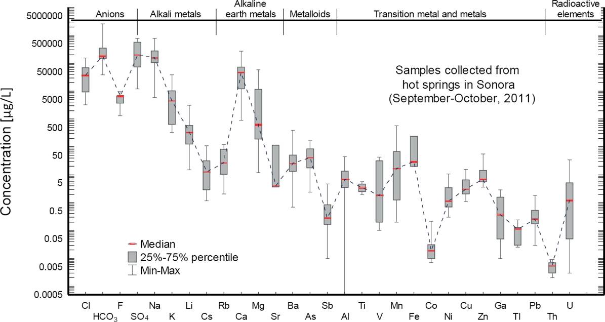
Figure 6 Statistical descriptive plot showing the main compositional features observed for major and trace elements measured in the hot spring samples of the Sonora geothermal system.
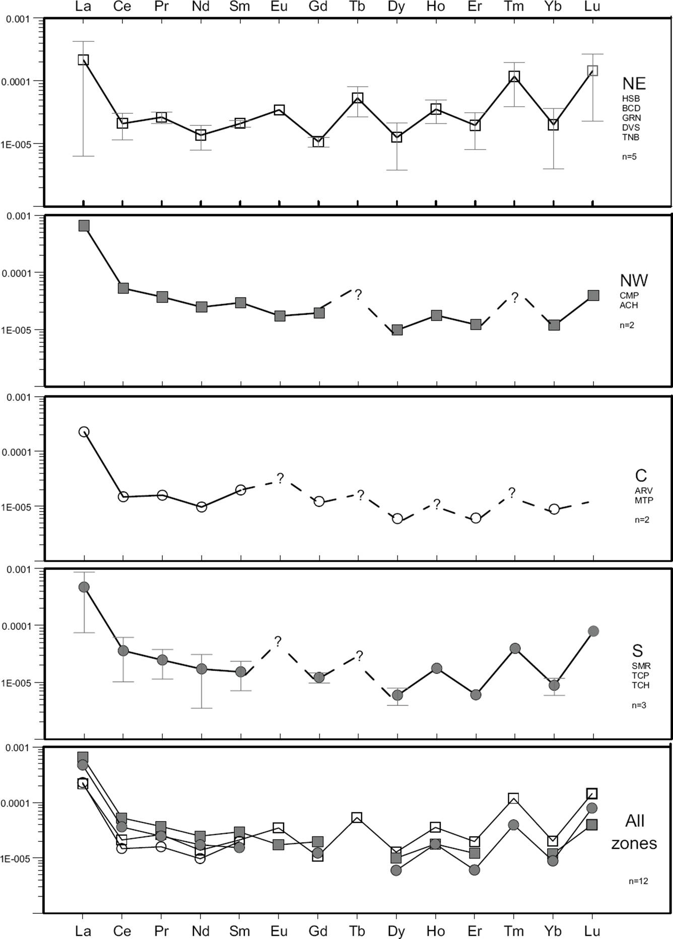
Figure 7 Rare Earth Element (REE) patterns normalized to chondrite values for the hot spring waters of the NE, NW, C and S zones. All the symbols correspond to the mean value for each zone each zone; bars indicate minimum and maximum values.
The statistical descriptive plot (Schoeller type) clearly indicates that the hot spring waters are mainly depleted in the major elements F-, Cl-, K+ and Li+, and enriched in HCO3 -, SO4 2-, Na+ and Ca2+ (Figure 6). Regarding the trace element contents, depletions were mainly observed for Cs, Sr, Sb, V, Co and Tl, whereas enrichments were mostly given for Rb, Ba, As, Al, Mn and Fe. A high chemical mobility from the host rock to the fluid (fractionation) was mainly observed in Mn, Fe, Sr, As, Rb, Ba, including the light REE (La and Ce). Intermediate and heavy REE were immobile elements that were not partitioned into the fluid due to the alkaline pH conditions (pH>6) that dominated most of the WRI and water mixing processes observed in the hydrothermal system.
An interesting geochemical signature of the NE hot spring waters is the zig-zag pattern observed for the REE, with positive and negative anomalies of Eu and Gd, respectively. This REE pattern is roughly observed for the NW and S hot spring waters, whereas for the C zone appears almost as a flat pattern (see Figure 7).
As seen in Table 5, boron (a highly mobile and conservative element) was not measured in the hot spring waters because it is generally present in high-temperature geothermal systems (Aggarwal et al. 2000; Gurav et al., 2016). According to the local WRI processes (i.e., fluid fractionation or chemical mobility) that occur in the hydrothermal system of Sonora, the non-volatile elements characterized as non-reactive or conservative compounds were mainly associated to the contents of Cl, Li, Rb, and Cs, whereas the reactive or geoindicator elements were typified by the concentrations of major cations (Na, K, Ca, Mg), and SiO2.
A multivariate statistical analysis of the linear relationships for all the physicochemical parameters, major and trace elements was applied by using a correlation matrix (Table 6a and 6b). Correlations among these variables provided valuable information of the major hydro-geochemical processes that controlled part of the chemical signatures found in the hot spring waters. Applying the methodology suggested by Bevington and Robinson (2003) for a small data sample (n=12), correlation coefficients of r>0.823 provide an acceptable correlation for a confidence level of 99.9%, whereas r values ranging from 0.5 to 0.7 shows a moderate correlation among the parameters. From this analysis, the physicochemical parameters (EC and TDS) resulted in high correlations (r>0.82) for both the cation (Na+, K+, Li+ and Ca2+) and anion (SO4 2- and HCO3 -) contents (see Table 6a). From the correlation matrix, it was found that TDS and EC of the hot spring waters were mainly controlled by Li+-HCO3 - and Na+-SO4 2- ions, respectively.
Table 6a Correlation matrix of the physicochemical parameters and the major ion content in water samples from hot springs in central-eastern Sonora (the best correlations were considered for r>0.823, n=12, and α=0.001; according to Bevington and Robinson, 2002).
| Tsup | pH | EC | TDS | Na+ | K+ | Li+ | Ca2+ | Mg2+ | F- | Cl- | SO4 2- | HCO3 - | SiO2 | |
|---|---|---|---|---|---|---|---|---|---|---|---|---|---|---|
| Tsup | 1 | |||||||||||||
| pH | 0.1394 | 1 | ||||||||||||
| EC | -0.0702 | -0.5959 | 1 | |||||||||||
| TDS | -0.2129 | -0.6138 | 0.9822 | 1 | ||||||||||
| Na+ | -0.0661 | -0.4781 | 0.9826 | 0.9555 | 1 | |||||||||
| K+ | -0.1432 | -0.7160 | 0.9743 | 0.9825 | 0.9298 | 1 | ||||||||
| Li+ | -0.1609 | -0.6080 | 0.9751 | 0.9862 | 0.9630 | 0.9782 | 1 | |||||||
| Ca2+ | -0.2125 | -0.7647 | 0.8888 | 0.9296 | 0.8001 | 0.9445 | 0.8932 | 1 | ||||||
| Mg2+ | -0.4920 | -0.6833 | 0.6345 | 0.7447 | 0.5223 | 0.7480 | 0.6825 | 0.8634 | 1 | |||||
| F- | 0.7683 | 0.1240 | -0.0758 | -0.2197 | -0.0005 | -0.1615 | -0.1091 | -0.3301 | -0.6555 | 1 | ||||
| Cl- | 0.3691 | -0.1229 | 0.1628 | 0.0301 | 0.1672 | 0.0849 | 0.0502 | 0.0055 | -0.2811 | 0.4418 | 1 | |||
| SO4 2- | 0.3390 | -0.4811 | 0.8687 | 0.7777 | 0.8649 | 0.7943 | 0.7785 | 0.6761 | 0.2948 | 0.2784 | 0.2654 | 1 | ||
| HCO3 - | -0.4551 | -0.5937 | 0.8682 | 0.9448 | 0.8290 | 0.9148 | 0.9242 | 0.9125 | 0.8717 | -0.4523 | -0.1709 | 0.5370 | 1 | |
| SiO2 | 0.6667 | -0.0311 | 0.3925 | 0.2657 | 0.4652 | 0.3117 | 0.3540 | 0.0977 | -0.2971 | 0.7749 | 0.2784 | 0.6837 | 0.0074 | 1 |
Table 6b Summarized correlation matrix of the major and trace elements in water samples from hot springs in central-eastern Sonora (the best correlations were considered for r>0.823, n=12, and α=0.001; according to Bevington and Robinson, 2002).
| Na+ | K+ | Li+ | Ca2+ | SO4 2- | HCO3 − | Be | Ti | Mn | Fe | Ge | Rb | Y | Zr | Nb | |
|---|---|---|---|---|---|---|---|---|---|---|---|---|---|---|---|
| Na+ | 1 | ||||||||||||||
| K+ | 0.9298 | 1 | |||||||||||||
| Li+ | 0.9630 | 0.9782 | 1 | ||||||||||||
| Ca2+ | 0.8001 | 0.9445 | 0.8932 | 1 | |||||||||||
| SO4 2- | 0.8649 | 0.7943 | 0.7785 | 0.6761 | 1 | ||||||||||
| HCO3 − | 0.8290 | 0.9148 | 0.9242 | 0.9125 | 0.5370 | 1 | |||||||||
| Be | 0.7941 | 0.7532 | 0.7662 | 0.5827 | 0.8649 | 0.5426 | 1 | ||||||||
| Ti | 0.7530 | 0.7008 | 0.7106 | 0.5317 | 0.8620 | 0.4255 | 0.8287 | 1 | |||||||
| Mn | 0.8537 | 0.9061 | 0.9166 | 0.8962 | 0.6793 | 0.9014 | 0.6514 | 0.6427 | 1 | ||||||
| Fe | 0.8591 | 0.9246 | 0.9379 | 0.9211 | 0.5930 | 0.9787 | 0.5491 | 0.5196 | 0.9595 | 1 | |||||
| Ge | 0.8587 | 0.8040 | 0.8179 | 0.6241 | 0.9028 | 0.5590 | 0.9354 | 0.9327 | 0.7200 | 0.6176 | 1 | ||||
| Rb | 0.8446 | 0.8446 | 0.8038 | 0.7270 | 0.9518 | 0.5696 | 0.8770 | 0.9048 | 0.7164 | 0.6266 | 0.9442 | 1 | |||
| Y | 0.8039 | 0.9064 | 0.9167 | 0.9314 | 0.6050 | 0.9445 | 0.6310 | 0.5365 | 0.9431 | 0.9515 | 0.6408 | 0.6380 | 1 | ||
| Zr | 0.9102 | 0.8308 | 0.9022 | 0.7520 | 0.7311 | 0.8434 | 0.6992 | 0.6259 | 0.8800 | 0.8738 | 0.7019 | 0.6506 | 0.8559 | 1 | |
| Nb | 0.8705 | 0.9332 | 0.9500 | 0.9196 | 0.6253 | 0.9691 | 0.5840 | 0.5805 | 0.9621 | 0.9946 | 0.6521 | 0.6573 | 0.9584 | 0.8901 | 1 |
On the other hand, the cation concentrations (Na+, K+, Li+, and Ca2+) were highly correlated with most of the major elements found in the hot spring waters, as well as with the trace elements Mn, Fe, Ge, Rb, Y, Zr, and Nb. In relation to the anion compositions, SO4 2- resulted in a good correlation with Be, Ti, Ge, and Rb; whereas the HCO3 - concentrations were well correlated with Mn, Fe, Y, Zr, and Nb. Among trace elements, Mn, Fe, Y, and Nb showed the highest correlation coefficients.
Hydrogeochemistry (fluid classification)
Major components of the hot spring waters were plotted in a Piper plot (Figure 8). As seen from this diagram, the geothermal fluids produced in the hot springs of the Central zone (MTP and ARV) were classified as calcium and magnesium-bicarbonate (Ca-Mg-HCO3) waters, compositions that are in concordance with the sedimentary formation from where they emerge after WRI and mixing processes. The waters produced in the NW (ACH and CMP), two NE (GRN and TNB), and S (TCP, SMR and TCH) hot springs were mostly grouped as sodium-sulphate (Na-SO4) waters, whereas those fluids coming from three hot springs from the NE hydrothermal zones (BCD, HSB and DVS) were mainly characterized as sodium-bicarbonate (Na-HCO3) waters. As seen in Figure 8, the hot spring waters of the Central zone (MTP and ARV) have entirely different chemistry compared to the other springs, which indicates that these waters probably come from a totally different fluid source or reservoir. The major-ion data of the remaining hot spring waters very well matches with more systematic chemical signatures of a geothermal system of low-to-medium temperature, which mostly dominates along the NW, NE and S zones.

An additional geochemical classification of fluids is also represented in the Cl-HCO3-SO4 ternary diagram proposed by Giggenbach (1988). According to this diagram (Figure 9), the hot spring waters produced at the Central (MTP and ARV), South (TCP and SMR) and NE (BCD and DVS) zones may be roughly classified as peripheral waters (i.e., bicarbonate and diluted chloride waters with a low concentration of sulphates) with a tendency toward volcanic waters; whereas the remaining hot spring waters fall on the plot section of “steam heated waters” due to the relative high proportion of sulphates found in the samples (NW: ACH and CMP; NE: HSB, GRN and TNB; and the anomalous TCH sample of the S zone, which seems to be the most representative water sample by its higher surface temperature, and typified as a mix chloride-sulphate or volcanic water). Some water samples (e.g. GRN, TNB, and HSB) exhibited anomalous alkaline pH between 6.8 and 9, which could not be strictly considered as characteristic of “steam heated waters”. The classification of these samples is difficult to understand because it would be expected to have acid waters (pH<3) instead of slightly acid sulphate waters with pH >6. To support these anomalous geochemical signatures, some recent geochemical findings reported in the literature on the possible origin of these geothermal fluids are discussed.
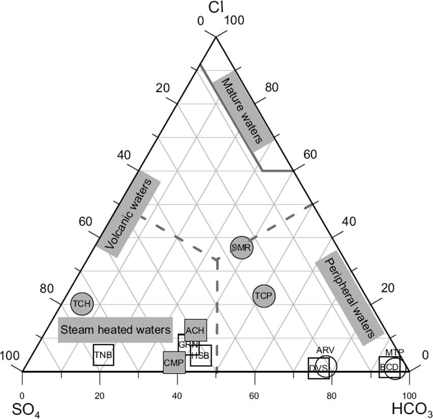
Figure 9 Ternary diagram showing the variation of major anions (Cl-, SO4 2- and HCO3 -) in the hot spring waters.
Smith et al. (2010) pointed out that in magmatic-hydrothermal and associated geothermal systems, acid magmatic fluids (with pH<3) are usually typified by a high concentration of sulphates, which are commonly discharged from hot springs nearby to the vent of active (degassing) volcanoes. However, these authors also describe that slightly acid geothermal fluids (with pH>5) may be found close to lateral outflows some distance away from the main degassing vent. Under these conditions, “alkaline sulphate waters” might be discharged with a diluted ionic composition.
Furthermore, reactions among dissolved carbon dioxide and host rocks tend to form HCO3 -, the concentration of which is probably affected by permeability and lateral flow. As a result of this process, hot springs that are fed directly from the reservoir tend to exhibit the lowest HCO3 - concentrations (which is actually characterized by the TCH water sample: 38.6 mg/kg and the highest surface temperature). This enables the HCO3 -/SO4 2- ratio to be used as an indicator of flow direction. The flow of a fluid away from the upflow yields the suitable conditions for rock-water reaction, and therefore for an increase of HCO3 -. This, combined with the loss of H2S by rock-water reactions with increased lateral flow, leads to an increase in the HCO3 -/SO4 2- ratios away from the upflow zone with values ranging from 0.07 (TCH) to 2 (TCP) for hot springs located at low altitudes of ~400 m a.s.l. (S zone), and from 0.25 to 11 for hot springs situated at an interval of altitudes between 600 and 900 m a.s.l. (NW, NE, and C zones).
Additionally, and to support the detection of relative high proportions of sulphates in six water samples from the NW, NE and S zones (see Figure 9), three precipitated salt samples were collected in situ at the CMP, TCH and TNB hot springs, and analysed by X-Ray Diffraction (XRD) for determining the major mineral compositions. The results of these XRD analyses show that the minerals that precipitated from the CMP waters were mainly characterized as quartz (SiO2), thenardite (Na2SO4), and calcite (CaCO3), whereas those for TCH and TNB hot springs were typified as gypsum (CaSO4 .2H2O), and a mixture of thenardite (Na2SO4) and halite (NaCl), respectively (see Figure 10). Taking into account these XRD analyses, the composition of these hot spring waters (as a product of the interaction with or dissolution of these precipitated minerals) may be in agreement with the unusual concentrations of sulphates reported for these water samples (see Figure 9). All these classification signatures are mostly in agreement with the grouping inferences obtained from the Piper diagram.
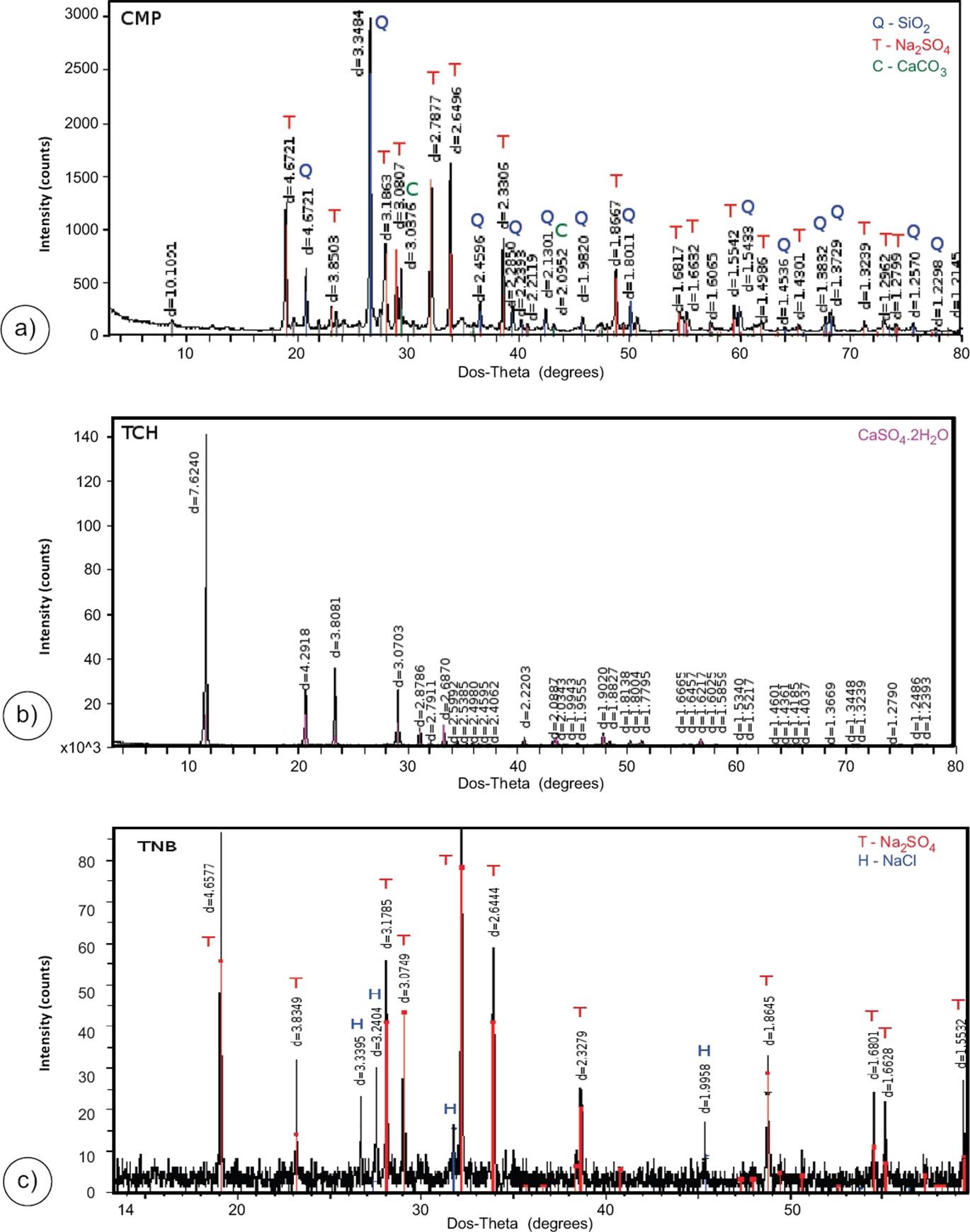
Figure 10 XRD diffractograms of precipitated salt samples collected at the (a) CMP, (b) TCH and (c) TNB hot springs.
Ternary diagram of Li-Rb-Cs
The lithium concentrations in the hot spring waters varied between 0.66 and 3.1 mg/kg for the NE zone, whereas lower concentrations were found for the NW and S hydrothermal zones which ranged from 0.41 to 0.47 mg/kg, and from 0.17 to 0.53 mg/kg, respectively. Hot spring waters that emerge from the C zone show the lowest lithium concentrations (0.020 mg/kg). On the other hand, Rb concentrations were mostly the highest for the NE zone (up to 123 µg/kg), whereas for the NW and S zones, intermediate concentrations ranging from 25.40 to 35.80 µg/kg, and from 9.95 to 75.3 µg/kg, respectively, were found. The lowest concentrations of Rb were actually measured for the C zone. In relation to Cs, a systematic composition pattern was identified for all the hydrothermal zones (ranging from 4 to 123 µg/kg for the NE; from 12.50 to 28.80 µg/kg for the NW; from 3.16 to 16.4 µg/kg for the S; and from 2.67 to 3.16 for the C). This pattern is shown in the ternary diagram of Li-Rb-Cs (Figure 11). The plot shows chemical signatures related to a group of hot spring samples falling between the basalt and rhyolite rock boundaries, which are well characterized by K/Rb and K/Cs ratios ranging from 109 to 192, and from 112 to 567, respectively. According to Goguel (1983), it is assumed that these waters may interact with illite at temperatures between 190 and 210 oC.
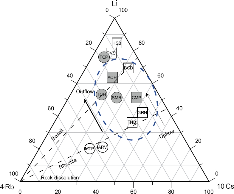
Figure 11 Ternary diagram showing relative Li, Rb, and Cs contents in the hot spring waters. Outflow and upflow are schematically shown. Dotted area comprises the group of hot spring samples falling between the basalt and rhyolite rock boundaries, which limit the waters thay may have interacted with illite at temperatures between 190 and 210 °C (Goguel, 1983).
On the other hand, the enrichment of Rb in presence of low concentrations of Li seems to indicate that these hot waters reached temperatures around 210 °C at the reservoir conditions before mixing with shallow cold waters during their ascent towards the surface. As a result of these chemical signatures, the study of the ternary diagram of Li-Rb-Cs may also be used as a secondary proxy indicator for inferring the theoretical reservoir temperatures of the Sonora hot spring waters.
Isotopic analyses
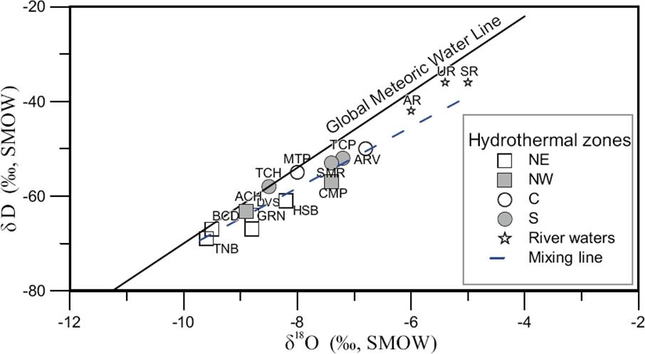
The water isotopic composition (D/H and 18O/16O) is considered as a conservative signature, and it is a good geochemical indicator for inferring water origin, mixing and evaporation processes, as well as a proxy for identifying the intensity degree of water rock interaction when the rock permeability is low (Bahati et al., 2005). Results of the isotopic analyses (δ18O and δD) for the hot spring samples collected in Sonora are reported in Table 5. The isotopic composition of these waters shows an approximated dispersion of 2.7 units (from -6.9 to -9.6 with an accuracy of ±0.08 ‰) for 18O/16O, and 19 units (from -50 to -69 with an accuracy of 0.9 ‰) for D/H.
All these data points are shown in a δ18O - δD plot (Figure 12), where the Global Meteoric Water Line (GMWL) is also represented. Isotopic data from waters of three nearby rivers Ures (UR), Aconchi (AR) and Sonora (SR) are also plotted as reference of the local isotopic composition of cold water in the study area. As seen in Figure 12, the isotopic compositions of some hot spring waters lie near to the GMWL, particularly those corresponding to the hot springs TCH and MTP from the S and C hydrothermal zones, respectively. The remaining samples (TNB, BCD, ACH, GRN, DVS, HSB, CMP, SMR, TCP, and ARV) show a clear shift for both δ18O and δD, which is described by the dashed mixing line (Figure 12). This signature is generally the result of mixing with isotopically heavier water. The hot spring waters are probably a mixture of waters similar to the most depleted local groundwaters with a composition that results from the intersection of the mixing line with the GMWL, and an isotopically heavier water not identified in the study zone.
Fluid geothermometry
Pseudo-equilibrium temperature estimates were obtained by the application of seven solute geothermometers (Na/K: 3, K-Mg, Na-K-Ca, Na-Li, and SiO2). The results of these calculations are reported in Table 7.
Table 7 Deep reservoir temperatures estimated from solute geothermometers (°C).
| Zone | Sample | Tsup | TNa/K 1 | TNa/K 2 | TNa/K 3 | TK−Mg 4 | TNa−K−Ca 5 | TNa/Li 6 | TSiO2 7 |
|---|---|---|---|---|---|---|---|---|---|
| NW | ACH | 50.8 ± 4.1 | 137.5 ± 42.8 | 143.2 ± 34.4 | 98.4 ± 8.3 | 101.0 | 200.1 | 157.6 ± 25.4 | 123.3 ± 1.0 |
| NW | CMP | 45.5 ± 0.2 | 111.3 ± 38.9 | 117.7 ± 31.4 | 69.1 ± 7.4 | 71.7 | 321.3 | 146.4 ± 24.4 | 108.4 ± 0.9 |
| NE | BCD | 34.8 ± 3.9 | N.A. | 68.8 ± 25.9 | N.A. | 69.5 | 83.1 | 101.1 ± 20.7 | 101.9 ± 0.9 |
| NE | HSB | 35.9 ± 0.4 | N.A. | 27.7 ± 21.8 | N.A. | 72.1 | 52.4 | 54.6 ± 17.2 | 97.8 ± 0.9 |
| NE | GRN | 46.1 ± 1.2 | 142.3 ± 43.5 | 147.9 ± 35.0 | 103.9 ± 8.5 | 101.5 | 136.4 | 147.7 ± 24.5 | 119.5 ± 1.0 |
| NE | TNB | 49.8 ± 1.0 | 147.3 ± 44.3 | 152.7 ± 35.6 | 109.7 ± 8.6 | 104.0 | 229.1 | 136.4 ± 23.6 | 132.8 ± 1.1 |
| NE | DVS | 29.3 ± 0.5 | 161.8 ± 46.6 | 166.8 ± 37.4 | 126.5 ± 9.2 | 76.6 | 147.8 | 178.3 ± 27.2 | 111.9 ± 1.0 |
| C | MTP | 30.9 ± 2.9 | N.A. | N.A. | N.A. | 40.9 | 21.7 | 144.9 ± 24.3 | 69.2 ± 0.7 |
| C | ARV | 40.0 ± 0.2 | N.A. | N.A. | N.A. | 39.8 | 187.3 | 104.5 ± 20.9 | 81.9 ± 0.8 |
| S | TCP | 41.5 ± 7.2 | 118.2 ± 39.9 | 124.4 ± 32.2 | 76.7 ± 7.6 | 76.6 | 116.2 | 117.6 ± 22.0 | 107.2 ± 0.9 |
| S | SMR | 31.4 ± 0.2 | 132.1 ± 42.0 | 138.0 ± 33.8 | 92.3 ± 8.1 | 61.9 | 118.5 | 115.0 ± 21.8 | 95.2 ± 0.9 |
| S | TCH | 63.1 ± 0.6 | 142.4 ± 43.5 | 148.0 ± 35.0 | 104.0 ± 8.5 | 112.3 | 126.8 | 128.7 ± 22.9 | 118.8 ± 1.0 |
1 Fournier (1979); 2,6,7Verma and Santoyo (1997); 3Díaz-González et al. (2008); 4Giggenbach (1988); 5Fournier and Truesdell (1973). N.A. — the geothermometer equations were not applied because the estimates provided unrealistic temperature values.
Na/K geothermometer
A good agreement among the temperatures calculated by three different versions of the Na/K geothermometer was roughly obtained. The Na/K ratios ranged between 20.7 and 48.1 for the spring waters of the NW, NE (except BCD: 143 and HSB: 467), and S zones, which provided reliable temperature approaches for the reservoir. These estimates must be considered as lower limits of the reservoir temperatures because the chemical signatures of the hot spring waters show evidence of mixing with shallow groundwater, as well as the interaction with surface precipitated minerals. In this context, hot spring waters that are subject to conductive cooling, lateral flow or near surface reactions tend to exhibit high Na/K ratios (between 12.3 and 60) for temperatures ranging from 100 °C to 200 °C (Nicholson, 1993; O’Brien, 2010). It is well-known that the prediction capability of this geothermometer at temperatures below to 200 °C (i.e., with Na/K ratios ranging from 13 to 27) provide greater uncertainties than those ratios (ranging between 3 and 13) corresponding to high temperatures (between 200 °C and 340 °C). This limitation of the Na/K geothermometer is due to the long WRI times needed for achieving equilibrium between Na and K in controlled laboratory experiments at low-to-medium temperatures (<200 °C; Pérez-Zarate et al., 2015).
The TNaKVS97 geothermometer systematically provided higher temperature estimates, whereas lower temperature values were computed with the TNaKDSR08 geothermometer. Anomalous higher temperatures of 328±62 °C and 462±87 °C were also calculated for the ARV and MTP hot spring, respectively (values that were excluded from the Table 7). These unrealistic temperature estimates were expected because such samples exhibited anomalous chemical and isotopic signatures (probably caused by the high content of Mg), in comparison with the remaining water samples. On the other hand, temperatures corresponding to the HSB and BCD (which are alkaline together with TCP) hot springs could not be determined with confidence due to the complex chemical and isotopic signatures that revealed some mixing or diluting effects caused by the local hydrogeochemical processes recorded by these samples (see Figures 8-12).
To analyse the anomalous temperature estimates, the Na/K concentration ratios of the geothermal fluids were computed. The highest values of the Na/K ratios were obtained for the HSB and BCD (466.7 and 142.9, respectively), whereas the lowest values correspond to the MTP and ARV hot springs (1.4 and 3.4, respectively). High Na/K ratios may suggest either a preferential leaching of Na or removal of some of the K in the form of secondary alteration products (Giggenbach, 1988), which could be confirmed in future prospection studies by collecting fresh and altered rock samples for analysing the presence of alteration minerals (e.g., muscovite, microcline). Low Na/K ratios were associated to a prediction of unrealistic high temperatures. These geochemical anomalies may be attributed either to ion exchange processes among clay minerals or simply to the lack of equilibrium conditions between solutes and alteration minerals (which is evidenced by the presence of incompletely equilibrated spring waters, probably due to mixing or dilution processes); see the classical Na-K-Mg geothermometer diagram (Figure 13). In this triangular plot, a fast equilibrating process is represented by the K/Mg geothermometer, whereas the slow equilibrating process is given by the Na/K geothermometer (Giggenbach 1988).
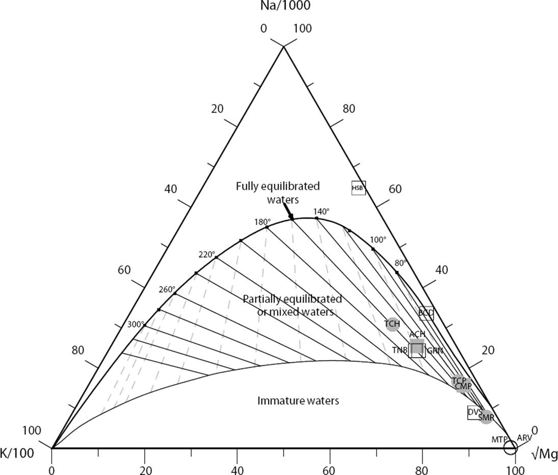
Figure 13 Ternary equilibrium diagram showing the relative Na, K and Mg contents for all the hot spring samples collected in the four hydrothermal zones of the Sonora geothermal system (based on Giggenbach, 1988).
By excluding the extreme temperatures inferred from ARV and MTP (the highest temperature estimates), and from HSB, and BCD thermal springs (the lowest temperature estimates) (see Table 7), and after applying a geochemometric analysis based on outliers detection/rejection under the assumption of a normal distribution, the mean reservoir temperature predicted with the TNaKVS97 equation for the hot springs CMP, GRN, SMR, TCP, TCH, DVS, TNB, and ACH was 142±16 °C (see Figure 14).
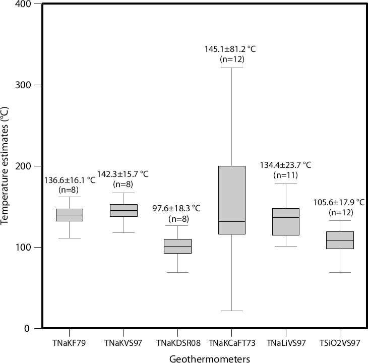
Figure 14 Results of the statistical outlier detection/rejection analysis applied for all the solute geothermometers, and mean reservoir temperatures estimated by each solute geothermometer.
For the outlier detection/rejection, the univariate analysis applied the Dixon, Grubbs, skewness and kurtosis statistical tests at the 99% confidence level by using the computer code UDASYS of Verma et al. (2013). A distribution map showing the most attractive geothermal potential zones (NW and NE) based on these reservoir temperature approaches is shown in Figure 15a. According to this map, lower reservoir temperatures are mainly distributed in the S hydrothermal zone (SMR, TCP and TCH).
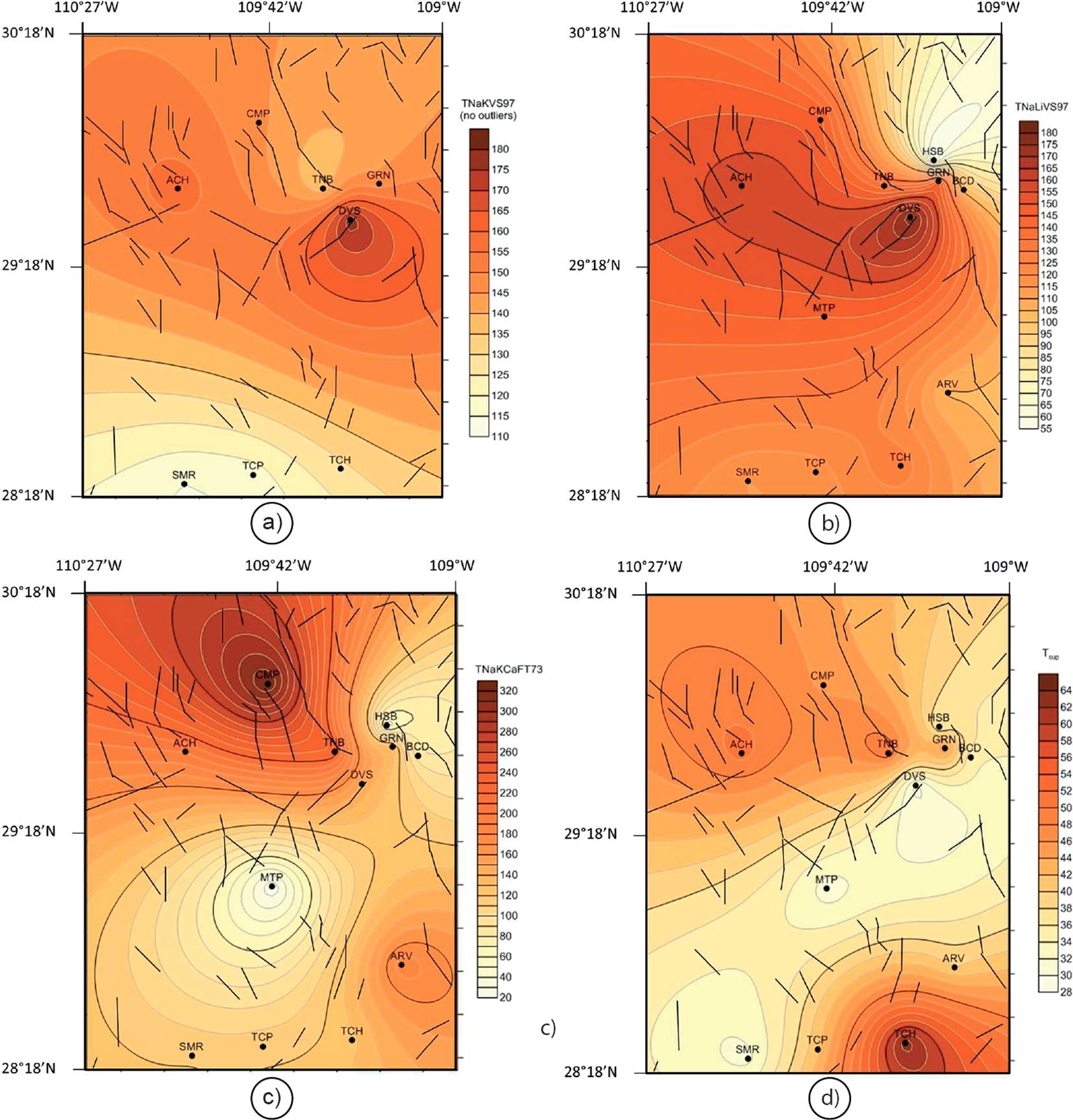
Figure 15 Distribution map showing the most attractive geothermal zones (NW and NE) based on the most reliable reservoir temperature approaches (inferred from the solute geothermometers): a) TNaKVS97; b) TNaLiVS97; and c) TNaKCaFT73. The distribution of the surface temperatures measured in the four hydrothermal zones is also plotted as reference (d).
Na-Li geothermometer
Na/Li ratios were calculated after converting the ion concentrations into mol/kg units. Na/Li ratios for all the hot spring waters ranged from 76.5 to 230.7. Reservoir temperatures were estimated using the corresponding TNaLiVS97 equations by considering their molality constraints (chlorides) indicated in Table 3. After applying the appropriate TNaLiVS97 equations, estimates of reservoir temperatures for nearly all the hydrothermal zones under evaluation ranged from 101±21 °C to 178±27 °C. An anomalous lower temperature of 55±17 °C was estimated for the HSB hot spring. For identifying the origin of this anomalous temperature, the Na/Li ratios of all the water samples were analysed. The highest value of this ratio was obtained for the HSB hot spring (Na/Li=576.3). High Na/Li ratios may suggest either a preferential leaching of Na or a removal of some alteration minerals of Li (e.g., Li-chlorite, Fouillac and Michard, 1981).
Following the same methodology used with the TNaKVS97 geothermometer, the geochemometric analysis based on outliers detection/rejection was again applied. From this statistical analysis, it was found that the anomalous lower temperature estimated for the HSB hot spring belongs to the same statistical sample of the TNaLiVS97 temperature estimates (i.e., it was not an outlier value). Therefore, the mean reservoir temperature inferred from the TNaLiVS97 indicated values of 134±24 °C (Figure 14). A distribution map showing the obtained TNaLiVS97 reservoir temperatures, and the most attractive geothermal potential zones is shown in Figure 15b. Similarly to the contour map of TNaKVS97 temperatures, lower reservoir temperatures were associated to the S hydrothermal zone (i.e., SMR, TCP and TCH).
Na-K-Ca geothermometer
Before applying the Na-K-Ca (TNaKCaFT73) geothermometer, √Ca/Na ratios were first computed. Such ratios ranged between 2.07 and 4.65, which provided acceptable reservoir temperatures for the hydrothermal zones under evaluation. These temperature approaches varied between 116 °C and 148 °C.
Anomalous higher temperatures of 321 °C, 229 °C, and 200 °C were calculated for the CMP, TNB, and ACH hot springs, respectively. On the other hand, lower temperatures of 22 °C, 52 °C and 83 °C for the MTP, HSB and BCD hot spring waters were respectively estimated mainly due to the low Ca concentrations observed in these samples. In order to analyse these temperature estimates, the √Ca/Na ratios of the hot spring waters were analysed. Highest values of √Ca/Na ratios were measured for the ARV and MTP hot springs (53.96 and 170.77, respectively), whereas the lowest values were determined in HSB and BCD (0.57 and 0.99, respectively). High √Ca/Na ratios may suggest either a preferential leaching of Ca (e.g. in carbonated rock formations) or a removal of some of the Na in the form of secondary alteration products (e.g., NaSO4). Low √Ca/Na ratios may be also due to either Ca precipitation (e.g., travertine) or to the lack of equilibrium between solutes and alteration minerals observed in these zones.
After applying the geochemometric analysis (based on outliers detection/rejection under the assumption of a normal distribution), a mean reservoir temperature from the TNaKCaFT73 was estimated as 145±81 °C (Figure 14). A distribution map showing the geothermal potential zones (NW and NE) from the reservoir temperatures predicted by the TNaKCaFT73 is presented in Figure 15c, which also agrees with the temperature distribution field indicated by the TNaKVS97.
SiO 2 geothermometer
The use of the TSiO2VS97 geothermometer for the determination of reservoir temperatures predicted mean values of 106±18 °C, which were systematically lower than those reservoir temperatures estimated by the Na/K, Na/Li, and Na-K-Ca geothermometers.
Estimation of the mean reservoir temperature
A two-way analysis of variance (ANOVA), with one sample by group at α=0.05 (or 5%), was applied to the reservoir temperature estimates (excluding the rejected values from the outliers analysis, Table 7). The ANOVA test was iteratively applied for evaluating both the statistical differences among temperature estimates for hot springs and solute geothermometers under the following two strict cases of analysis: (i) if the reservoir temperature estimates of the hot spring waters were statistically the same among hot springs (Ho 1 ); and (ii) if there are statistical significant differences among the predictions made by the solute geothermometers (Ho 2 ). When both strict conditions were statistically fulfilled, the estimation of the mean reservoir temperature was then calculated. Table 8 summarises the results obtained from the iterative ANOVA analysis. After three cycles of this analysis, the following results were obtained:
1) Cycle # 1: Statistical hypotheses — Ho1: all temperature estimates among the hot springs are statistically the same; whereas Ha1: not all temperature estimates among the hot springs are statistically the same; For α=0.05 and the obtained p-value=0.225, Ho1 cannot be rejected (see Table 8). Ho2: all temperature estimates among the geothermometers are statistically the same; Ha2: not all temperature estimates among the geothermometers are statistically the same. For α=0.05 and the obtained p-value=8.5×10⁻⁴, Ho2 is rejected;
2) Cycle # 2: Statistical hypotheses (after removing all the temperature estimates predicted by the TNaKDSR08 geothermometer because these data were identified as the lowest estimates according to the outlier detection algorithm) — According to the calculated F values and following the same statistical methodology, it is concluded that Ho1 cannot be rejected; whereas the Ho2 is rejected; and,
3) Cycle # 3: Statistical hypotheses (after removing all the temperature estimates predicted by the TSIO2VS97 geothermometer with the same statistical argument) — According to the calculated F values and following the same statistical methodology, it is concluded that both hypotheses Ho1 and Ho2 cannot be rejected, and therefore, the mean reservoir temperature may be estimated as 149±40 °C using the temperature estimates of the ACH, TCP, TNB, TCH, CMP, DVS, GRN, and SMR hot springs (see Table 8). This conclusion highlights the importance of applying suitable geothermometric tools at each geothermal site.
Table 8 Two factor variance analysis with one sample by group applied to the equilibrium temperature estimates (α=0.05).
| Sample | TNaKF79 | TNaKVS97 | TNaKDSR08 | TNaKCaFT73 | TNaLiVS97 | TSiO2VS97 |
|---|---|---|---|---|---|---|
| ACH | 137.5 | 143.2 | 98.4 | 200.1 | 157.6 | 123.3 |
| CMP | 111.3 | 117.7 | 69.1 | 321.3 | 146.4 | 108.4 |
| GRN | 142.3 | 147.9 | 103.9 | 136.4 | 147.7 | 119.5 |
| TNB | 147.3 | 152.7 | 109.7 | 229.1 | 136.4 | 132.8 |
| DVS | 161.8 | 166.8 | 126.5 | 147.8 | 178.3 | 111.9 |
| TCP | 118.2 | 124.4 | 76.7 | 116.2 | 117.6 | 107.2 |
| SMR | 132.1 | 138 | 92.3 | 118.5 | 115 | 95.2 |
| TCH | 142.4 | 148 | 104 | 126.8 | 128.7 | 118.8 |
| Iterative Cycle # 1 | ||||||
| Variation origin | Square addition | Degrees of freedom | Square means | F | Probability | F critical value |
| Rows | 10242.63 | 7 | 1463.23 | 1.43 | 0.22536 | 2.28 |
| Columns | 27740.86 | 5 | 5548.17 | 5.42 | 0.00085 | 2.49 |
| Error | 35853.67 | 35 | 1024.39 | |||
| Total | 73837.16 | 47 | ||||
| Iterative Cycle # 2 | ||||||
| Variation origin | Square addition | Degrees of freedom | Square means | F | Probability | F critical value |
| Rows | 10673.48 | 7 | 1524.78 | 1.29 | 0.29097 | 2.35 |
| Columns | 14693.01 | 4 | 3673.25 | 3.1 | 0.03092 | 2.71 |
| Error | 33082.75 | 28 | 1181.52 | |||
| Total | 58449.25 | 39 | ||||
| Iterative Cycle # 3 | ||||||
| Variation origin | Square addition | Degrees of freedom | Square means | F | Probability | F critical value |
| Rows | 11504.36 | 7 | 1643.48 | 1.1 | 0.39 | 2.48 |
| Columns | 7306.84 | 3 | 2435.61 | 1.63 | 0.21 | 3.07 |
| Error | 31326.45 | 21 | 1491.73 | |||
| Total | 50137.66 | 31 | ||||
Iterative Cycle # 1: Statistical hypotheses — Ho1: all temperature estimates among the hot springs are statistically the same, i.e., come from the same statistical sample; whereas Ha1: not all temperature estimates among the hot springs are statistically the same; For α=0.05 and the obtained p-value=0.225, Ho1 cannot be rejected. It is therefore concluded that all the temperature estimates among the hot springs are statistically the same. Ho2: all temperature estimates among the geothermometers are statistically the same; Ha2: not all temperature estimates among the geothermometers are statistically the same. For α=0.05 and the obtained p-value=8.5E-04, Ho2 is rejected. It is also concluded that not all the temperature estimates among the geothermometers are statistically the same.
Iterative Cycle # 2: Statistical hypotheses (after removing TNaKDSR08 temperature estimates) — According to the F calculated values and following the same statistical methodology, it is concluded that Ho1 cannot be rejected; whereas the Ho2 is rejected.
Iterative Cycle # 3: Statistical hypotheses (after removing TSIO2VS97 temperature estimates) — According to the F calculated values and following the same statistical methodology, it is concluded that Ho1 and Ho2 cannot be rejected, and therefore, the mean reservoir temperature may be estimated as 149±40 oC.
Mixing geochemical model
Taking into consideration the water mixing processes evidenced from the classification diagrams (Figures 8, 9, 11) and the D/H and 18O/16O plot (Figure 12), a mixing geochemical model based on a silica and fluid enthalpy plot was applied for inferring the water composition and temperature at the original reservoir conditions. The silica content of ascending hot spring waters (which fall outside of the full equilibrium curve: Figure 13) and their corresponding fluid enthalpy were plotted in Figure 16. The influence of a conductive cooling was quantitatively examined for determining the mixing degree with colder waters.
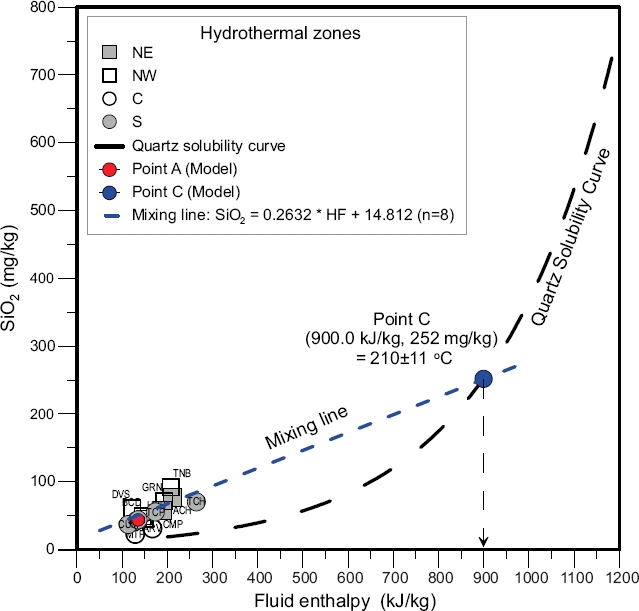
Figure 16 SiO2-enthalpy mixing model and mixing line obtained for the hot spring waters of the Sonora geothermal system.
After applying the model, it was inferred that the original reservoir conditions indicate a deep reservoir temperature of 210±11 °C, together with a silica content of 300±27 mg/kg, and a fluid enthalpy of 950±85 kJ/kg (see the blue point C in Figure 16). This reservoir temperature is higher than those estimates predicted from the solute geothermometers (Table 7), and it may be considered as the maximum reservoir temperature of the Sonora geothermal system.
According to the Li-Rb-Cs diagram (Figure 11), this reservoir temperature of 210±11 °C is in good agreement with the temperature that controls the illite mineral interaction, and the temperature interval inferred from the K/Rb and K/Cs ratios. All the geochemical signatures observed at deep reservoir conditions reflect the degree of mixing of the waters during their ascent towards the surface.
Fluid-mineral equilibria
For evaluating the pseudo-equilibrium state that actually exhibit most of the waters sampled in the twelve hot springs, the Na-K-Mg diagram was again examined (Figure 13). This diagram associates the hydrothermal fluids with their most probable reservoir temperatures. As seen in Figure 13, most of the hot spring waters fall in the region of mixed waters or partial equilibrium (e.g., ACH and CMP from the NW zone; BCD, GRN, TNB, and DVS from the NE zone; and TCP, SMR and TCH from the S zone). Some exceptions were given by water samples falling outside or in the limits of the full equilibrium line (HSB and BCD from the NE zone), and two remaining water samples located in the section of immature waters (MTP and ARV from the C zone). This geochemical shift was probably caused by the loss of some ions (e.g., K) by these two water samples. Another possible cause may be related to the total dissolved carbonate concentration, which in the specific case of the HSB and BCD water samples comprises both HCO3 - and CO3 2- species). The total carbonate concentration may also be influenced by the CO2 partial pressure in the deep geothermal fluid (P CO2) and the pH (Nicholson, 1993). The loss of CO2 during boiling processes normally raises the pH of the fluid by consuming protons through the involved reactions (i.e., the water usually becomes more alkaline, as in the case of HSB and BCD samples which exhibited the highest pH values of 9.0 and 8.5, respectively; see Table 5).
The lack of equilibrium with the surrounding host rocks is also confirmed by the mixing model (see Figure 16), and explained either as a result of a mixing between hydrothermal waters and colder shallow fluids during the path towards the surface, or simply due to meteoric waters coming from different sources or river waters (Figure 11; e.g., MTP and ARV). The origin of the HSB hot spring water (located above the full equilibrium line in Figure 13) is probably related to mixing with some evaporated water sources (Figure 11).
From the thermal point of view, most of the water samples were distributed in the partial equilibrium region where the reservoir temperatures vary from 75 °C to 175 °C, most of them falling close to the 150 °C isotherm, which seems to be the lower limit of the reservoir temperatures of the geothermal system.
Using 150 °C and 200 °C as rounded-off reservoir temperatures (or min-max values) and the Geochemist’s Workbench software, geochemical equilibrium modelling based on fluid-mineral stability diagrams was carried out. The dominant species and mineral phases that are stable over this temperature interval (i.e., mineral stability diagrams of the primary and secondary minerals for these reactions) were investigated. The following water-rock (mineral) systems were found as the major chemical and mineral signatures underlying the geothermal system under study (see the mineral stability diagrams in Figures 17a and 17b):
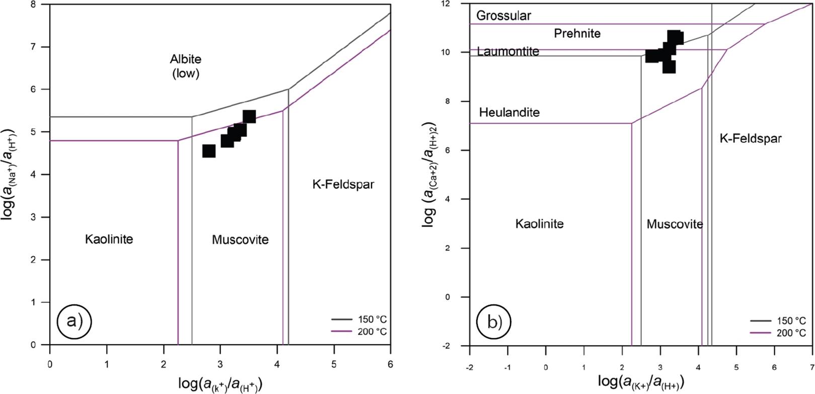
Figure 17 Fluid-mineral stability diagrams obtained for the (a) Na2O-K2O-Al2O3-SiO2-H2O and (b) CaO-K2O-Al2O3-SiO2-H2O systems.
1) A Na2O-K2O-Al2O3-SiO2-H2O system, which exhibited ionic exchange between Na and K that seems to be controlled either by the albite/muscovite or the albite/K-feldspar mineral interactions under metastable equilibrium conditions. This system reflects the hydrothermal alteration of primary plagioclase minerals in agreement with the following reaction:
The discharge fluid composition tends to be placed along an extension from either the albite/K-feldspar limit through the muscovite field, or through phases chemically similar like sericite and illite (Hedenquist, 1991). This behaviour can be interpreted as the result of the primary dissolution of feldspars in the reservoir under metastable equilibrium conditions between albite and K-feldspar (Torres-Alvarado, 2002). As seen in Figure 17, the albite and muscovite (K-mica as illite or sericite) interaction shows much better equilibrium conditions at temperatures close to 200 °C than those data corresponding to 150 °C (e.g., Henley and Ellis, 1983; Hedenquist et al., 2000). These interactions were mainly observed in the hot spring waters of the NW (ACH and CMP), NE (BCD, GRN and TNB), and S (SMR and TCH) zones.
2) A CaO-K2O-Al2O3-SiO2-H2O system, where the ionic exchange between Ca and K is described by the prehnite-laumontite-muscovite mineral assemblage (see Figure 17). These WRI processes seem to be associated with the hot spring waters from the NE (DVS and HSB), and S (TCP) zones. Laumontite is a Ca-rich zeolite typically observed in some geothermal fields at temperatures between 170 °C and 250 °C (Reyes, 1990; Torres-Rodríguez, 2000). It would be expected that hot spring waters in equilibrium with laumontite indicate the existence of a reservoir with a temperature interval between 120 °C and 210 °C (Reyes, 1990).
Most of these minerals belong to mineral assemblages of low grade metamorphism (Liou et al., 1985). This WRI signature seems to indicate that, according to the regional geology of the study area, the hot spring waters are reaching the chemical equilibria at the contact zones between the plutonic rocks (from the Laramide Batholith) and the tectonic basins (i.e., at regional fault zones under the influence of those plutonic rocks and low-grade metamorphism rocks). The lithological units that represent the former metamorphic features are the intermediate to acidic volcanic rocks from the Tarahumara Formation. The interpretation of the most probable pseudo- or equilibrium conditions among the hot spring waters and the mineral assemblages in the Na2O-K2O-Al2O3-SiO2-H2O and CaO-K2O-Al2O3-SiO2-H2O systems seem to be in a good agreement with the expected reservoir temperatures observed in the hydrothermal zones, and the theoretical thermal stability of hydrothermal minerals by Henley and Ellis (1983) and Hedenquist et al. (2000): Figure 18.

Figure 18 Thermal stability of various hydrothermal minerals (modified after Hedenquist et al., 2000 and Henley and Ellis, 1983). (a) Mineral assemblages associated to pH and temperature; (b) Mineral assemblages associated only to temperature. Dashed orange lines indicate the pH and estimated temperature values prevailing in the hot spring waters reported this study (purple and red dashed lines correspond to minimum and maximum estimates respectively).
Conclusions
The presence of hot springs, Quaternary volcanism, and tectonic activity at the east-central Sonora state (Mexico) was reported in this prospection study. A field work campaign for the collection of representative samples from twelve hot springs was carried out. From chemical and isotopic analyses of these samples, a study of the major chemical and isotopic signatures of fluids produced in this low-to-medium temperature geothermal system was inferred.
Hydrothermal waters with the highest surface temperatures (up to 63.1 °C) were mainly associated to hot springs emanating on granite rocks (in the basin and range limits marked by regional faults), whereas the lowest surface temperatures (up to 29.3 °C) were mostly observed for hot springs that emanate on recent sediments (alluvium) within the valleys. Based on the chemical signatures of the hot spring waters (major and trace elements), depletion (F-, Cl-, K+, and Li+ and Cs, Sr, Sb, V, Co and Tl) and enrichment (in HCO3 -, SO4 2-, Na+ and Ca2+ and Rb, Ba, As, Al, Mn and Fe) in fluid compositions were identified. A high chemical mobility from the host rock to the fluid was also observed in Mn, Fe, Sr, As, Rb, Ba, and the light REE (La and Ce).
The interpretation of hydrogeochemistry classification diagrams mostly indicated the presence of sodium-sulphate (Na-SO4) waters in the North (NW: ACH and CMP; and NE: GRN and TNB) and South (TCP, SMP and TCH) hydrothermal zones; whereas calcium and magnesium-bicarbonate (Ca-Mg-HCO3) waters were found for the Central zone (MTP and ARV). Two hot spring waters located in the NE (BCD, HSB and DVS) zone were characterized as sodium-bicarbonate (Na-HCO3) type waters. The signatures of stable isotopes (δ18O and δD) indicate a meteoric origin for four hot spring waters (NE: BCD and TNB; S: TCH; and C: MTP), which lie near to the global meteoric water line; whereas a small shift for both isotopes was observed in the rest of the samples (NW: ACH and CMP; NE: HSB, GRN and DVS; C: ARV; and S: TCP and SMR). This small δ18O shift typified a mixing line which was used as a proxy to discriminate waters with a different isotopic signature.
After applying a geochemometric analysis (based on outlier detection/rejection and ANOVA), the mean reservoir temperature was estimated as 149±40 °C. By considering the mixing process among hot spring and shallow colder waters, the temperature of the reservoir was corrected by applying a conductive cooling model, from which a deep reservoir temperature of 210±11 °C was inferred. Both temperatures 149±40 °C and 210±11 °C are considered with confidence as the minimum (realistic) and maximum (optimistic) reservoir temperatures of the Sonora geothermal system. Using some approaches to these reservoir temperatures (150 °C and 200 °C), as the most probable equilibrium temperatures (min-max), it was found that the hot spring waters are in equilibrium with mineral assemblages of the Na2O-K2O-Al2O3-SiO2-H2O (NW: ACH-CMP; NE: BCD-GRN-TNB; and S: SMR and TCH) and CaO-K2O-Al2O3-SiO2-H2O (NE: DVS-HSB; and S: TCP) systems. These minerals are proposed as representative mineral assemblages of low-grade metamorphism.
The integrated geochemical model here proposed enabled the evolution of the Sonora hydrothermal reservoir to be described, where a deep fluid circulation characterised by low-to-medium temperatures (t<200 °C) dominates in the system. Based on this geochemical model, it is concluded that the hot spring waters from the geothermal system of east-central Sonora have the potential to be used not only for heat direct use, but also for electricity production through plants of binary cycle, which are suitable to be safely operated with fluid temperatures between 100 °C and 180 °C and with very low environmental issues.

