Hydrological modeling of ungauged wadis in arid environments using GIS: a case study of Wadi Madoneh in Jordan

 

Modelo hidrológico de wadis sin datos de aforo en ambientes áridos usando GIS: un caso de estudio en Wadi Madoneh, Jordania

 

Nezar Hammouri^1,* and Ali El–Naqa²

 

1 Department of Earth and Environmental Sciences, Hashemite University, P.O.Box 150459, Zarqa, Jordan.

2 Department of Water Management and Environment, Hashemite University, P.O.Box 150459, Zarqa, Jordan.* nezar@hu.edu.jo

 

Manuscript received: August 1, 2006
Corrected manuscript received: March 27, 2007
Manuscript accepted: April 8, 2007

 

ABSTRACT

Runoff is one of the most important hydrological variables used in most of the water resources applications. Reliable prediction of runoff from land surface into streams and rivers is difficult and time consuming to obtain for ungauged basins. However, Remote Sensing (RS) and Geographic Information System (GIS) technologies can augment to a great extent the conventional methods used in rainfall–runoff studies. These techniques can be used to estimate the spatial variation of the hydrological parameters, which are useful as input to the rainfall–runoff models. The main objective of this study was to model the rainfall–runoff process in a selected ungauged basin for the purpose of groundwater artificial recharge. This model simulation was carried out using an hydrological modeling system assisted by GIS. Two model runs were carried out using precipitation data of the Intensity–Duration–Frequency (IDF) curves at Zarqa rainfall station for 10 years and 50 years return periods. With the first model run, the total direct runoff volume and the peak discharge for the 10 years return period were estimated to be 151,000 m³ and 5.43m³/s, respectively. For the 50 years return period, the total direct runoff volume and the peak discharge were estimated to be 280,000 m³ and 12.77m³/s, respectively. The model was optimized against observed runoff data, measured during a storm event that occurred between the 2nd and the 4th of April, 2006. The flow comparison graph indicates that the calibrated model fits well with the observed runoff data, with a peak–weighted root mean square error (RMS) of less than 2%. This calibration was performed by applying different curve numbers in the simulated model. It was possible to obtain a reasonable match between the simulated and the observed hydrographs.

Key words: surface runoff, ungauged basin, rainfall–runoff model,digital elevation model, geographic information system, Wadi Madoneh, Jordan.

 

RESUMEN

El escurrimiento es una de las variables hidrológicas más importantes que se emplea en la mayoría de los usos de los recursos de agua. La obtención de una predicción confiable del escurrimiento superficial hacia corrientes y ríos en cuencas sin datos de aforo es un proceso difícil que consume mucho tiempo. Sin embargo, las tecnologías de percepción remota y los Sistemas de Información Geográfica (SIG) pueden complementar en gran medida a los métodos convencionales en estudios de lluvia–escurrimiento. Estas técnicas pueden ser aplicadas para estimar la variación espacial de los parámetros hidrológicos que se emplean en modelos de lluvia–escurrimiento. El objetivo principal de este estudio fue modelar el proceso de lluvia–escurrimiento en una cuenca sin datos de aforo con el propósito de evaluar su potencial para la recarga artificial del agua subterránea. Este modelo de simulación se realizó usando un sistema de modelado hidrológico apoyado por SIG. Se obtuvieron dos modelos usando datos de precipitación de las curvas de Intensidad–Duración–Frecuencia (IDF) de la estación de Zarqa para períodos de retorno de 10 años y de 50 años. Con el primer modelo, el volumen directo total del escurrimiento y la descarga máxima, o pico, para el período de retorno de 10 años fueron estimados en 151,000 m³ y 5.43m³/s, respectivamente. Para un período de retorno de 50 años, se estimó un volumen directo total del escurrimiento de 280,000 m³ y una descarga máxima de 12.77m³/s. El modelo fue optimizado contra datos observados de escurrimiento, medidos durante una tormenta que ocurrió entre el 2 y el 4 de abril de 2006. El gráfico de comparación del flujo indica que el modelo calibrado presenta un buen ajuste con los datos observados de escurrimiento, puesto que el error estándar ponderado (peak weighted root mean square error) es menor que 2%. Esta calibración se realizó aplicando diversos números de curvas en la simulación. Fue posible obtener un ajuste razonable entre los hidrogramas simulados y los observados.

Palabras clave: escurrimiento superficial, cuenca sin datos de aforo, modelo lluvia–escurrimiento, modelos de elevación digital, sistemas de información geográfica, Wadi Madoneh, Jordan.

 

INTRODUCTION

Jordan has turned to the use groundwater to satisfy the growing demand of water, at the expense of exceeding the safe yield and overexploiting the country's aquifers. In 1994, Jordan launched a program to explore the use of groundwater artificial recharge with the aim to offset some of the problems caused by this overexploitation. The preliminary site selection for groundwater artificial recharge was accomplished by the use of a geographic information system (GIS). Hydrologic information was spatially encoded and processed to yield the most promising locations in Jordan. These locations should have a surplus water resource, available aquifer space and acceptable land use practices. To generate a prioritized list of potential sites, a multi–criteria approach was used, based on different factors such as the need for water in a basin, water quality of recharge or host water, value in use of recharged water, and potential ecologic impacts. Two sites were selected on the basis of this analysis: the Wadi Butom (Azraq Governorate) and the Wadi Madoneh (Zarqa Governorate).

Runoff is one of the most important hydrological variables used in water resources studies. Reliable prediction of direct runoff for ungauged basins is difficult and time consuming. Conventional models for predicting stream discharge require considerable hydrological and meteorological data. Remote sensing and Geographic Information Systems (GIS), in combination with appropriate rainfall runoff models, provide ideal tools for the estimation of direct runoff volume, peak discharge and hydrographs (Miloradov and Marjanovic, 1991; Demayo and Steel, 1996; Bellal et al., 1996). The role of remote sensing in runoff estimation is generally to provide a source of input parameters for the models. Satellite data can provide thematic information on land use, soil, vegetation, drainage, etc., which, combined with conventionally measured climatic parameters (precipitation, temperature, etc.) and topographic parameters (elevation and slope), constitute the necessary input data for the rainfall–runoff models. The information, extracted from remote sensing and other sources, can be stored as a georeferenced database in a GIS. The system provides efficient tools for data input into databases, retrieval of selected data for further processing, and software modules that can analyze or manipulate the retrieved data in order to generate the desired information in a specific form (Miloradov and Marjanovic, 1991).

This study was focused on the Wadi Madoneh site to explore the surface water potential for groundwater artificial recharge using a Geographic Information Systems (GIS) and the Hydrologic Modeling System (HMS) of the Hydrologic Engineering Center (HEC). The HEC (1998) model was chosen for the simulation of rainfall–runoff using the Soil Conservation Service (SCS) curve number method, which was developed in the United States for small basins (USDA, 1986; USACE, 2000). The HEC–HMS rainfall–runoff model was used to estimate direct runoff volume, peak discharge and to construct synthetic hydrographs for an ungauged basin. In practice, the design of the artificial recharge structures is not intended to capture all runoff from all storm events in the basin areas, as it may be planned for large dams. Rather, the conceptual design for artificial recharge is to capture volumes of water that have low sediment content and can be feasibly and quickly recharged to the groundwater aquifer. Consequently, only runoff volumes of less than 500,000 m³, which would be generated by storm events of less than 40 mm precipitation, would be suitable for recharge (SAIC, 1996).

 

DESCRIPTION OF THE WADI MADONEH BASIN

The Wadi Madoneh site is located in the vicinity of the confluence of Wadi Madoneh with Wadi Ishshe, approximately eight kilometers southeast of the city of Ruseifa and nine kilometers south of the city of Zarqa. The city is about 15 km east of Amman and is readily accessible by asphalt paved roads. Directly to the east and south of the site begins the broad expanse of uninhabited or sparsely inhabited land, which extends eastward from Amman toward the town of Azraq (Figure 1). The bed elevations are between 700 m to 720 m above sea level, and hill top elevations range between 820 m and 850 m above sea level. The immediate vicinity of the site and upstream areas is generally flat within the bed and flood plain of the wadi; slopes may range up to about 5% (SAIC, 1996). The site area is undeveloped and generally inhabited; some houses are located in the site surroundings. The surface geology of the site is characterized by the outcropping of karstified and fractured limestone of the Wadi Sir Massive Limestone (A7) (Figure 2); the exposures of this unit are prominent along the slopes and hill slopes in the site area. The A7 formation is the last unit of the Ajlun Group (A1–A7), and is overlain by the Umm Ghudran Chalk Marl and the Amman Silicified Limestone of the Balqa Group (Rimawi, 1985).

The principal aquifer to be recharged beneath the Wadi Madoneh is the Wadi Sir Formation (A7), which is a major source of groundwater in Jordan. At depths below the A7 aquifer lie the A4 and A2 aquifer systems. In the vicinity of the site, the A7 aquifer is unconfined. The site is located within the recharge area for the A7 aquifer. Depth to the groundwater in the A7 aquifer across the site varies from 60 to 90 m. On the basis of regional data, general groundwater flow in the A7 aquifer located within the vicinity of the site is assumed to be toward the east–northeast. As part of the study, several wells in the vicinity of the site were rehabilitated for the purpose of measuring water levels and collecting some water quality samples.

Landuse in Wadi Madoneh basin is largely unclassified. However, the upstream sections of the basin area have been classified as cultivated or cultivable area. The climate of the area is characterized by hot summers and mild winters. The active precipitation stations in the surrounding area are located at Zarqa area. The precipitation data for the most recent 30 years period from 1973/1974 to 2002/2003 water years indicate that the average annual precipitation in the vicinity of the site and in the upstream basin ranges from approximately 120 to 150 mm. The annual average potential evaporation is approximately 1,075 mm. Soils in the study area are derived from the local bedrock. The two major soil texture classes are silty clay loam (SiCL) and silty loam (SiL) (Figure 3).

Wadi Madoneh and Wadi Ishshe drain an area of approximately 20 km² upstream of their confluence. Stream discharge data are not available for either wadi. Available information indicates that there are no recorded springs in the immediate vicinity of the site, which suggests that surface water flowing in the wadis is associated only with major precipitation events.

The nearest instrumented Wadi basin, with potentially similar precipitation and drainage characteristics to the Wadi Madoneh basin, is Wadi Sa'ida, located approximately 20 to 25 km to the north. Wadi Sa'ida was formerly instrumented with a continuous surface water recorder by the Ministry of Agriculture. The station has not been operational for several years and its period of record is limited. Consequently, stream discharge data for the station were not obtained.

 

SURFACE RUNOFF AND RAINFALL–RUNOFF MODELS

Runoff flow is composed of two main elements: base flow that has its origin in groundwater, and surface runoff, which is the accumulation of rainfall that drains to the stream. The basin characteristics that affect the base flow and the surface runoff include geology, soil type, vegetation cover, precipitation, drainage area and antecedent moisture condition (Bouwer, 1986; Zech et al., 1994; Bellal et al., 1996). Some generalized computer models for basin hydrology are able to compute sequences of daily or monthly stream flows for a given precipitation event, although these systems require considerable expertise, time and effort to be used effectively. However, the United States Soil Conservation Service (SCS) Curve Number (CN) method is relatively easy to use and yield adequate results (USDA, 1986; Schulze et al., 1992; Bellall et al., 1996). The SCS–CN is based on the hydrological characteristics of the soils in a watershed, type of soil cover, vegetation coverage, and surface storage potential. On the basis of the CN for the basin and the 24–hour precipitation events, an estimation of the potential runoff from the Wadi Madoneh/Wadi Ishshe catchment areas were obtained (SAIC, 1996). By using the hydrologic analysis techniques detailed in the SCS TR–55 Bulletin (Urban Hydrology for Small Watersheds), the 50–year, 24–hour precipitation events of 48 mm yielded an annual runoff of about 833,000 m³ (SAIC, 1996).

In this study, a hydrologic model was generated to estimate the runoff potential of Wadi Madoneh by using the Hydrologic Modeling System of the Hydrologic Engineering Center (HEC, 1998). This model was used to compare the estimated potential runoff volumes with the results obtained with the TR55 model (SAIC, 1996). The HEC–HMS model provides a variety of options for simulating precipitation–runoff processes. The hydrologic elements are arranged in a dendritic network, and computations are performed in an upstream–to–downstream sequence. Computations are performed in SI units. The execution of a simulation requires the specification of three sets of data. The first, labeled Basin Model, contains parameter and connectivity data for hydrologic elements; types of elements are: sub–basin, routing reach, junction, reservoir, source, sink and diversion. The second set, labeled Precipitation Model, consists of meteorological data and information required to process them. The model represents historical or hypothetical conditions. The third set, labeled Control Specifications, specifies time–related information for the simulation. A project can consist of a number of data sets of each type. A "run" is configured with one data set for basin model, precipitation model and control specifications.

To transfer the generated data layers as shape files into the HEC–HMS interface, the CRWR–PrePro utility was used (Olivera and Maidment,1998a, 1998b; Hellweger and Maidment, 1999). This utility, composed of ArcView Avenue scripts, was designed and developed to extract topographic, topologic and hydrologic information from digital spatial data of a hydrologic system, and to prepare ASCII files for the basin and precipitation components of HEC–HMS.

 

MODEL APPROACH

The model approach used to determine the runoff volume was the SCS–CN method (SCS, 1972). With this method, the precipitation excess is a function of cumulative precipitation, soil type, land use/cover and antecedent moisture. Considering the initial loss and the potential maximum retention, the precipitation excess can be calculated; the maximum retention and the basin characteristics are related through the curve number. The standard SCS curve number method is based on the following relationship between rainfall depth, P, and runoff depth, Q (USDA, 1986; Schulze et al., 1992):

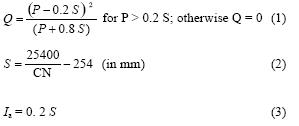
where: Q is the surface runoff (mm), P is the precipitation (mm), S is the soil retention (mm), I_a is the initial loss (mm), and CN is the curve number.

To obtain volumes, P and Q (in millimeters) must be multiplied by the basin area. The potential maximum retention (S) represents an upper limit for the amount of water that can enter the basin through surface storage, infiltration, and other hydrologic losses. For convenience, S is expressed in terms of a CN, which is a dimensionless basin parameter ranging from 0 to 100. A CN of 100 represents a limit condition for a perfectly impermeable basin with zero retention, where all the rainfall becomes runoff. A CN of zero conceptually represents the other extreme, with the basin trapping all the rainfall with no runoff regardless of the rainfall amount. The basin parameter CN can be determined from empirical information. The SCS has developed tables of initial curve number (CN_i) values as a function of the basin soil type and the land cover/use/condition. These are listed in Schulze et al. (1992). The hydrologic soil groups are defined in accordance to the standard SCS soil classification procedures, which establish a range from classification A for sand and aggregated silts with high infiltration rates, to classification D for soils that swell significantly when wet and have low infiltration rates. On the basis of the soil information for Wadi Madoneh basin and the visible ground coverage, a CN of 78 was chosen. A potential retention (S) of 71.64 mm was computed by applying Equation 2. The initial loss (I_a) was estimated to be 14.33 mm from Equation 3. These values were used in the model for the Wadi Madoneh basin.

To determine how the runoff is distributed over time we must introduce a time–dependent factor. The time–of–concentration (t_c) is used in the SCS methods. The t_c is most often defined as the time required for a particle of water to travel from the most hydrological remote point in the basin to the point of collection. There are several methods available for calculating t_c, one of them is the SCS Lag Method:

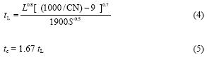
where t_c is the time of concentration (minutes); t_L is the watershed lag time (minutes); L is the length of longest watercourse (ft); S is the mean slope of the basin (%); and CN is the curve number.

 

INPUT DATA FOR THE HEC–HMS BASIN MODEL

The following procedure was adopted to construct a basin model for Wadi Madoneh basin. Figure 4 shows a schematic representation of the proposed model along with different input, output, and processing elements. The first step is preparing a Digital Elevation Model (DEM) (Stefan, 1996). In order to generate the DEM for the study area, a contour map in scale 1:50,000 was used to digitize the 50 m contour interval. With the aid of ArcMap GIS 9.0, these digitized contours were converted to a DEM with 80m cell size. Such DEMs include pits or ponds that should be removed before being used in hydrological modeling (Ashe, 2003). These are cells where water would accumulate when drainage patterns are being extracted. Pits are a sign of errors in the DEM arising from interpolation. These pits were removed by an algorithm known as SINK filling. This algorithm is built in the interface of the CRWR–PrePro utility.

After filling the DEM sinks, a flow direction map was computed by calculating the steepest slope and by encoding into each cell the eight possible flow directions towards the surrounding cells. Flow direction is then used to generate the flow accumulation map. The flow accumulation, generated by addressing each cell of the DEM, counts how many upstream cells contribute to flow through the given cell. Flow direction and accumulation maps are then used to delineate the stream network. The stream network can be divided into segments, which will determine the outlets of the basin. The generated stream network has a dendritic shape of third order.

The last step is the basin delineation process, which depends on the generated flow direction and accumulation map. Furthermore, it also depends on a user–specified number known as threshold (Djokic et al., 1997). This threshold determines the minimum number of pixels within each delineated sub–basin. A value of 5,000 was chosen to delineate the basin because the basin area is small, whereas a value of 1,000 was used to divide the Wadi Madoneh basin into four sub–basins. Figure 5 shows the generated sub–basins along with the stream network.

 

COMPUTATION OF HYDROLOGIC PARAMETERS

The sub–basin parameters (area, lag–time and average curve number) were calculated with the CRWR–PrePro utility (Maidment, 1992). Other parameters, needed for estimating the lag–time, such as length and slope of the longest flow path, were also calculated and stored in the sub–basin attribute table. These files, when opened in HEC–HMS, automatically create a topologically correct schematic network of sub–basins and reaches with hydrologic parameters. Table 1 shows the attribute table for the sub–basins with the calculated hydrologic parameters.

The following procedure was adopted to construct the rainfall–runoff model for the Wadi Madoneh basin. A schematic representation of the Wadi Madoneh network was created by dragging and dropping icons that represent hydrological elements, and connections between them were established. The hydrologic parameters for each sub–basin were entered using HEC–HMS sub–basin editor; required data consist of sub–basin area, loss rate method (SCS–CN method was used), transform method (SCS Unit Hydrograph method was used), and baseflow method (baseflow was set to zero for Wadi Madoneh). Considering that the time span of the storm event was short, it was assumed that evapotranspiration was zero.

A precipitation model is the next component of the HEC–HMS model. The intensity of rainfall was obtained from the Intensity–Duration–Frequency (IDF) curve of Zarqa rainfall station for two selected return periods:10 years and 50 years. For each time duration, the corresponding precipitation depth was computed as the product of intensity and duration. The precipitation data were entered for 10 years and 50 years return periods. Finally, the control specifications for a three–day simulation period (from the 2^nd to the 4th of April, 2006) were selected with 1 hour time interval.

Table 2 shows a summary of the computed direct runoff volume and peak discharge for each sub–basin in the simulated model. The peak discharge for the 24–hour design storm with a 10 years return period was 5.43 m³/s. Furthermore, the hydrographs for each sub–basin and for the basin outlet are shown in Figures 6 and 7, respectively. The amount of runoff that would have been suitable for feasible artificial recharge practices for the simulated periods ranged from 150,970 m³ to 279,700 m³.

 

MODEL CALIBRATION AND OPTIMIZATION

Model calibration is an essential process needed to assure that the simulation outputs are close to real observations. Once a model was developed and simulated for the initial parameter estimates, it was calibrated against known discharge runoff rates measured at the Zarqa station during a storm event that occurred between the 2nd and the 4th of April, 2006. The model calibration was done by adjusting the curve number values until the results matched the field data. The process was completed manually by repeatedly adjusting the parameters, computing, and inspecting the goodness of fit between the computed and observed hydrographs. The process can also be done automatically by using the iterative calibration procedure called optimization. The measure of the goodness of fit is the objective function (Kathol et al., 2003). HEC–HMS allows the user to calibrate the model to the best–fit condition by selecting various objective functions to provide the best calibration results (HEC, 2005). The objective function measures the variation between computed and observed hydrographs, and is equal to zero when the hydrographs are identical. The automated calibration was used to adjust initial losses, curve number and lag time to minimize the objective function value and to find optimal parameters. When manual validation of the observed and simulated hydrograph was not acceptable, initial parameters were adjusted to provide a better optimization target value for the optimization process (USACE, 2000). The objective function used was the peak–weighted root mean square error (RMS). This objective function gave greater weight to large errors and lesser weight to small errors, in addition of giving greater overall weight to error near the peak discharge.

The optimization procedure required the use of a search method for minimizing an objective function and finding optimal parameters. The search method used for this calibration was the univariate gradient method. This method evaluated and adjusted one parameter at a time while holding all other parameters constant. The search method estimates the optimal parameters but do not indicates which parameters had the greatest impact on the solution (Kathol et al., 2003). Besides evaluating the objective function for determining if the process produced an accurate calibration, graphical comparisons were made between the fit of the model and the actual measured data. Graphical comparisons of scatter plots and time series plots of residuals between computed and observed flow were used to visually inspect the results of the calibration (Kathol et al., 2003).

The storm event used to calibrate the model was chosen because of the goodness of fit for the basin. The function value for the peak RMS error was set at only 0.1. The values for the basin model parameters indicate that the CN had low sensitivity to changes in the function value. Therefore, any change in the CN value will slightly affect the overall function if all other variables are held constant. The curve number was set to an optimized value of 84.6. This is a reasonable value, as it is in the range of the CN values (78–86) estimated for other basins by the Water Authority of Jordan (WAJ).

The results of the difference in volume and peak runoff for the simulated model versus the observed model are included in Table 3. The values for time of peak runoff and the time of center of mass for the simulated and observed results are also included in that table. The results show that the model overpredicts volume and peak flow for the 10 and 50 years IDF.

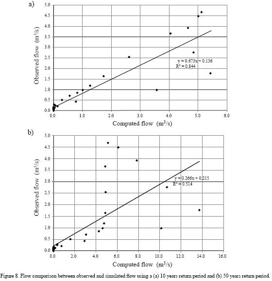
The flow comparison graph for the outlet of the Madoneh catchment area indicates how well the calibrated model fits the observed runoff data (Figure 7). Figure 8 shows a scatterplot between observed and simulated outflows. The results indicate that the model is not biased in overpredicting or underpredicting the simulated runoff.

 

RESULTS AND DISCUSSION

The purpose of this study was to explore the surface water potential for groundwater artificial recharge.Unfortunately, the study area is an ungauged basin, and information about surface runoff is critical for this purposes. Geographic Information Systems (GIS) and the hydrologic model HEC–HMS were used to simulate rainfall–runoff using the Soil Conservation Service (SCS) curve number method (see final simulation results in Table 2). The only available data to judge the quality of this simulation was a surface runoff measurement made by the Ministry of Water and Irrigation in April, 2006. For the calibration of the generated simulation, the measured peak flow of 4.68 m³/s was used to enhance the difference between the simulated and observed flow graph. Several curve number values ranging from 78 to 86 were used in this context to optimize the simulated hydrograph.

From the results of the hydrographs, the runoff volume, peak discharge and percent loss were determined. For the design storms with 10 years return period, the total precipitation of was 42.58 mm, the total loss was 34.59 mm, and the total rainfall excess (runoff) was 7.99 mm. While for the design storms with 50 years return period, the total precipitation of was 59.41 mm, the total loss was 42.00 mm and the total rainfall excess (runoff) was 17.41 mm.

The storm runoff analysis indicates that only precipitation events exceeding 14.3 mm within a 24–hour period would generate runoff. The total precipitation volume for water year 2005–2006 within the catchment area was approximately 3,125,000 m³ (WAJ internal files), while only about 5% of the total precipitation volume became runoff. Therefore, the expected runoff volume is about 156,000 m³. Consequently, based on conceptual considerations, only runoff volumes of less than 500,000 m³, which would be generated by storm events of less than 40 mm precipitation, would be suitable for recharge (SAIC, 1996).

 

CONCLUSIONS

Surface water flow resulting from runoff is the major source for the increasing fresh water demand. Determination of stream flow requires simulation of the contributing component into a hydrologic model. Hydrologic modeling requirs the determination of hydrologic parameters that are spatially and temporally variable. In such cases, GIS are the most powerful techniques used to estimate the model parameters, which generate models that simulate more or less the real conditions. The combination of these techniques with the SCS model makes the runoff estimate more reliable.

This study used the HEC–HMS precipitation–runoff model to predict the surface runoff that would occur in the Wadi Madoneh basin as result of different design storms. The model was calibrated against measured runoff events. The calibrated model yielded new parameter estimates for the basin. The flow comparison graph between simulated and observed flows indicates how the calibrated model fits the observed runoff data, and the flow residuals between the observed and the simulated data were obtained. The results indicate that the model is not biased in overpredicting or underpredicting the simulated runoff.

One of the major difficulties during this study was the lack or real surface runoff volumes. Unfortunately, most of Jordan basins are not equipped with surface water gauges to measure the surface runoff volumes during the rainy seasons. Therefore, in this study we presented a methodology for areas with similar conditions, which allows the estimation of surface runoff with acceptable accuracy.

 

REFERENCES

Ashe, R., 2003, Investigating runoff source area for an irrigation drain system using ArcHydro tools, in Proceedings of the Twenty–Third Annual ESRI User Conference, San Diego.        [ Links ]

Bellal, M., Sillen, X., Zeck, Y., 1996, Coupling GIS with a distributed hydrological model for studying the effect of various urban planning options on rainfall–runoff relationship in urbanised basins, in Kovar, K., Nachtnebel, H.P. (eds.), Application of Geographic Information Systems in Hydrology and Water Resources Management: International Association of Hydrological Sciences, Series of Proceedings and Reports, 235, 99–106.        [ Links ]

Bouwer, H., 1986, Intake rate: Cylinder infiltrometer, in Klute, A. (ed.), Methods of Soil Analysis, Part 1: Physical and mineralogical methods: Madison, WI, American Society of Agronomy and Soil Science Society of America, Agronomy Monograph No. 9, 825–844.        [ Links ]

Demayo, A., Steel, A., 1996, Data handling and presentation, in Chapman, D. (ed), Water Quality Assessments, A Guide to the Use of Biota, Sediments and Water in Environmental Monitoring: London, United Nations Educational, Scientific and Cultural Organization, World Health Oranization, United Nations Environment Programme, 2nd edition, Chapter 10, 511–612.        [ Links ]

Djokic, D., Ye, Z., Miller, A., 1997, Efficient watershed delineation using ArcView and spatial analyst, in Proceedings of the 17th Annual ESRI User Conference, San Diego, CA.        [ Links ]

Hellweger, F., Maidment, D.R., 1999, Definition and connection of hydrologic elements using geographic data: Journal of Hydrologic Engineering, 4(1), 10–18.        [ Links ]

Hydrologic Engineering Center (HEC), 1998, Hydrologic Modeling System, User's Manual: Davis, CA., United States Army Corps of Engineers, Institute for Water Resources, Hydrologic Engineering Center, 250 p.        [ Links ]

Hydrologic Engineering Center (HEC), 2005, Hydrologic Modeling System, User's Manual: Davis, CA., United States Army Corps of Engineers, Institute for Water Resources, Hydrologic Engineering Center, 260 p.        [ Links ]

Kathol, J. , Werner, H., Trooien, T., 2003, Predicting runoff for frequency based storms using a precipitation–runoff model, in North–Central Intersectional Meeting of the American Society of Agricultural Engineers (ASAE) and Canadian Society of Agricultural Engineers (CSAE), October 3–4, Fargo, North Dakota: St. Joseph, MI, ASAE Paper RRV03–0046.        [ Links ]

Maidment, D.R., 1992, Grid–based Computation of Runoff: A Preliminary Assessment: Davis, CA, Report Prepared for the Hydrologic Engineering Center, United States Army Corps of Engineers, Contract DACW04–92–P–1983.        [ Links ]

Miloradov, M., Marjanovic, P., 1991, Geographic information system in environmentally sound river basin development, in 3rd Rhine–Danube Workshop, Proceedings, 7–8 October: Delft, the Netherlands, Technische Universiteit Delft.        [ Links ]

Olivera, F., Maidment, D.R., 1998a, HEC–PrePro v. 2.0: An ArcView Pre–Processor for HEC's Hydrologic Modeling System, in Proceedings of the18th ESRI Users Conference, July 25–31, San Diego, CA.        [ Links ]

Olivera, F., Maidment, D.R., 1998b, GIS for hydrologic data development for design of highway drainage facilities: Transportation Research Record, 1625, 131–138.         [ Links ]

Rimawi, O., 1985, Hydrochemistry and isotope hydrology of groundwater and surface water in the north–east of Mafraq, Dhuleil, Hallabat, Azraq basin: Technische Universität München, PhD. thesis, 240 p.         [ Links ]

Science Application International Corporation (SAIC), 1996, Feasibility study of artificial recharge in Jordan: Amman, Ministry of Water and Irrigation, Unpublished report, 250 p.        [ Links ]

Schulze, R.E., Schmidt, E.J., Smithers, J.C., 1992, PC Based SCS Design Flood Estimates for Small Catchments in Southern Africa, SCS–SA User Manual: Pietermaritzburg, South Africa, University of Kwa–Zulu–Natal, Department of Agricultural Engineering, Report No. 40.        [ Links ]

Soil Conservation Service (SCS), 1972, National Engineering Handbook, Section 4, Hydrology: Washington DC, United States Department of Agriculture.        [ Links ]

Stefan, W.K., 1996, Using DEMs and GIS to define input variables for hydrological and geomorphological analysis, in Kovar, K., Nachtnabel, H.P. (eds.) Application of Geographic Information systems in Hydrology and Water Resource Management: International Association of Hydrological Sciences, Series of Proceedings and Reports, 235, 183–190        [ Links ]

United States Army Corps of Engineers (USACE), 2000, Hydrologic Modeling System HEC–HMS: Davis, CA, United States Army Corps of Engineers, Hydrologic Engineering Center, Technical Reference Manual, CPD–74B, 149 p.        [ Links ]

United States Department of Agriculture (USDA), 1986, Urban Hydrology for Small Watersheds: Springfield, VA, United States Department of Agriculture, Natural Resources Conservation Services, Conservation Engineering Division, Technical Release TR–55, 164 p.        [ Links ]

Zech, Y., Sillen, X., Debources, C., van Hauwaert, A., 1994, Rainfall–runoff modelling of partly urbanized watersheds: Comparison between a distributed model using GIS and other models sensitivity analysis: Water Science and Technology, 29(1–2), 163–170.        [ Links ]