Critical values for six Dixon tests for outliers in normal samples up to sizes 100, and applications in science and engineering

 

Valores críticos de seis pruebas de Dixon para datos desviados en muestras normales con tamaños de hasta 100 y aplicaciones en las ciencias e ingenierías

 

Surendra P. Verma^1,2* and Alfredo Quiroz–Ruiz¹

 

¹ Centro de Investigación en Energía, Universidad Nacional Autónoma de México, Priv. Xochicalco s/no., Col Centro, Apartado Postal 34, Temixco 62580, México.
* spv@cie.unam.mx

² Centro de Investigación en Ingeniería y Ciencias Aplicadas, Universidad Autónoma del Estado de Morelos, Av. Universidad No. 1001, Col. Chamilpa, Cuernavaca 62210, México

 

Manuscript received: September 21, 2005
Corrected manuscript received: March 10, 2006
Manuscript accepted: March 16, 2006.

 

ABSTRACT

In this paper we report the simulation procedure along with new, precise, and accurate critical values or percentage points (with 4 decimal places; standard error of the mean <0.0001) for six Dixon discordance tests with significance levels α = 0.30, 0.20, 0.10, 0.05, 0.02, 0.01, 0.005 and for normal samples of sizes n up to 100. Prior to our work, critical values (with 3 decimal places) were available only for n up to 30, which limited the application of Dixon tests in many scientific and engineering fields. With these new tables of more precise and accurate critical values, the applicability of these discordance tests (N7 and N9–N13) is now extended to 100 observations of a particular variable in a statistical sample. We give examples of applications in many diverse fields of science and engineering including geosciences, which illustrate the advantage of the availability of these new critical values for a wider application of these six discordance tests. Statistically more reliable applications in science and engineering to a greater number of cases can now be achieved with our new tables than was possible earlier. Thus, we envision that these new critical values will result in wider applications of the Dixon tests in a variety of scientific and engineering fields such as agriculture, astronomy, biology, biomedicine, biotechnology, chemistry, environmental and pollution research, food science and technology, geochemistry, geochronology, isotope geology, meteorology, nuclear science, paleontology, petroleum research, quality assurance and assessment programs, soil science, structural geology, water research, and zoology.

Key Words: Outlier methods, normal sample, Monte Carlo simulations, reference materials, earth.

 

RESUMEN

En este trabajo se presenta el procedimiento para la simulación junto con valores críticos o puntos porcentuales nuevos y más precisos y exactos (con 4 puntos decimales; el error estándar de la media <0.0001) de las seis pruebas de discordancia de Dixon y para los niveles de significancia α = 0.30, 0.20, 0.10, 0.05, 0.02, 0.01, 0.005 y para tamaños n de las muestras normales de hasta 100. Antes de nuestro trabajo, se disponía de valores críticos (con 3 puntos decimales) solamente para n hasta 30, lo cual limitaba seriamente la aplicación de las pruebas de Dixon en muchos campos de las ciencias e ingenierías. Con las nuevas tablas de valores críticos más precisos y exactos obtenidos en el presente trabajo, la aplicabilidad de las pruebas de Dixon (N7 y N9–N13) se ha extendido a 100 observaciones de una variable en una muestra estadística. Presentamos ejemplos de aplicaciones en muchos campos de ciencias e ingenierías incluyendo las geociencias. Estos ejemplos demuestran la ventaja de la disponibilidad de estos nuevos valores críticos para una aplicación muy amplia de esas seis pruebas de discordancia. Se esperan aplicaciones a un mayor número de casos en ciencias e ingenierías, estadísticamente más confiables que como era posible anteriormente. De esta manera, prevemos que los nuevos valores críticos resulten en aplicaciones de las pruebas de Dixon mucho más amplias en una variedad de campos de ciencias e ingenierías tales como agronomía, astronomía, biología, biomedicina, biotecnología, ciencia del suelo, ciencia nuclear, ciencia y tecnología de los alimentos, contaminación ambiental, geocronología, geología estructural, geología isotópica, geoquímica, investigación del agua y del petróleo, programas de aseguramiento y evaluación de calidad, paleontología, química, meteorología y zoología.

Palabras clave: Métodos de valores desviados, muestra normal, simulaciones Monte Carlo, materiales de referencia, pruebas de discordancia de Dixon, Ciencias de la Tierra.

 

INTRODUCTION

Two main sets of methods (Outlier methods and Robust methods; Barnett and Lewis, 1994) exist for correctly estimating location (central tendency) and scale (dispersion) parameters for a set of experimental data likely to be drawn, in most cases in science and engineering, from a normal or Gaussian distribution (Verma, 2005). The outlier scheme is based on a set of tests for normality (or detection of outliers) such as Dixon tests described here. However, caution is required when applying such outlier tests for samples that are not normally distributed. The alternative scheme for arriving at these parameters consists of a series of robust or accommodation approach methods (for location parameter: e.g., median, mode, Winsorized mean, trimmed mean, and mean quartile; and for scale parameter: e.g., interquartile range and median deviation; see Barnett and Lewis, 1994; Verma, 2005, or any standard textbook on statistics), all of which rely on not "taking into account" the outlying and other peripheral observations in a set of experimental data. These methods, although in use in many branches of science and engineering, will not be considered here any further because the main objective of this paper is to comment on and improve the applicability of six discordance tests, proposed by Dixon more than 50 years ago, which are still widely used as explained below.

Dixon (1950, 1951, 1953) proposed six discordance tests for normal univariate samples and estimated critical values or percentage points for these tests for sizes up to 30 and reported them to 3 decimal places. These tests were designated N7 and N9–N13 by Barnett and Lewis (1994). Dixon (1951) also stated that the estimated critical values for tests N7 (test statistic r₁₀ in this paper), N9 (statistic r₁₁), and N10 (statistic r₁₂)were "in error by not more than one or two units in the third (decimal) place", whereas those for tests Nil (statistic r₂₀), N12 (statistic r₂₁), andN13 (statistic r₂₂) were "believed to be accurate to within three or four units in the third (decimal) place".

These tests have been widely used –and are still in use– in the outlier–based scheme for correctly estimating the location and scale parameters (e.g., Thomulka and Lange, 1996; Freeman et al, 1997; Hanson et al, 1998; Verma et al, 1998; Woitge et al, 1998; Muranaka, 1999; Tigges et al. ,1999; Taylor, 2000; Hofer and Murphy, 2000; Buckley and Georgianna, 2001; Langton et al., 2002; Reed et al., 2002; Stancak et al, 2002; Yurewicz, 2004; Kern et al, 2005). However, these tests are applicable to only samples of sizes up to 30, which severely limits their application in many scientific and engineering fields, because, today, the number of individual data in a statistical sample has considerably increased (to much greater than 30) than was customary a few decades ago. Furthermore, Gawlowski et al. (1998) considered the Dixon tests for normal univariate samples as inferior to the Grubbs tests because the critical values for the former (quoted to only three significant digits, or 3 decimal places; Dixon, 1951) are less accurate than for the latter (quoted to four significant digits, or 3 or 4 decimal places depending on the critical values being >1 or <1; Grubbs and Beck, 1972). In fact, other reasons (see pp. 121–125 and p. 222 in Barnett and Lewis, 1994) might account for the relative efficiency of discordance tests than the one stated by Gawlowski et al. (1998).

The computation of new critical values for Dixon discordance tests through Monte Carlo simulations was motivated from multiple reasons: (1) The still wide use of these tests by researchers in many scientific and engineering fields (see selected references for the past ten years 1996–2005 cited above); (2) the availability of critical values for Dixon tests with 3 decimal places as compared to Grubbs tests with critical values with 3 or 4 decimal places; and most importantly (3) the inapplicability of these discordance tests to the actual data for numerous chemical elements in reference materials (RMs) in the field of (a) alloy industry (e.g., Roelandts, 1994); (b) biology (Ihnat, 2000); (c) biomedicine (Patriarca et al, 2005); (d) cement industry (Sieber et al, 2002); (e) food industry (In't Veld, 1998, Langton et al, 2002); (f) environmental research (Dybczynski et al., 1998; Gill et al., 2004; Holcombe et al., 2004); (g) rock geochemistry (e.g., Guevara et al, 2001); and (h) soil science (Dybczynski et al., 1979; Hanson et al., 1998; Verma et al, 1998), as well as to experimental data in numerous other scientific and engineering applications as will be explained later in this paper.

We included all six discordance tests (N7 and N9–N13; see pp. 218–236 of Barnett and Lewis, 1994), initially proposed by Dixon (1950,1951,1953), for simulating new, precise, and accurate critical values for n up to 100 (number of data in a given statistical sample, n = 3 (1) 100 for test N7, i.e., for all values of n between 3 and 100; n = 4(1)100 for tests N9 and Nil; n = 5(1)100 for tests N10 and N12; and n = 6(1)100 for test N13). The minimum number of data to be tested in a given sample (i.e., the minimum sample size) varies from 3 to 6 depending on the type of statistics to be computed (Table 1).

In this paper, we outline the simulation procedure and present new critical values for all six discordance tests and their comparison with the available literature critical values for n up to 30. We also highlight applications to evaluate experimental data in different science or engineering fields, including many branches of earth sciences.

 

SIX DIXON DISCORDANCE TESTS (N7 AND N9–N13)

Assume a univariate data set (a random sample from a normal population) of n observations represented by an array: x₁, x₂, x₃,..., x_n_₂, x_n_₁ x_n. If we arrange these data in ascending order, from the lowest to the highest observations, we may call the new array as: x₁, x₂, x₃,...,x_n_₂, x_n_₁ x_n where x₍₁₎ is the lowest observation and x_(n) is the highest one.

Tests N7, N9, and N10 are discordance tests for an extreme outlier (x_(n) or x₍₁₎) in a normal sample with population variance (σ²) unknown, whereas tests N11–N13 are for two extreme observations (either the upper–pair x_(n), x_(n–1) or the lower–pair x₍₁₎, x₍₂₎) in a similar normal sample. The corresponding test statistics are given in Table 1. As an example, the test statistic for test N7 is:

 

Suppose x_(n) is an outlier, i. e., it appears unusually far from the rest of the sample. The procedure for testing x_(n) includes first the computation of the statistic TN7 (equation 1) for an actual data set under evaluation. It is said that the value x_(n)is under evaluation, i.e., tested to see if it was drawn from the same normal population as the rest of the sample (null hypothesis H₀), or it came from a different normal sample (with a different mean or a different variance or both), i.e., if it happens to be a discordant outlier (alternate hypothesis H₁).

The computed value of test statistic TN7 is then compared with the critical value (percentage point) for a given number of observations n and at a given confidence level (CL) or significance level (SL or a), generally recommended to be 99% CL or 1% SL (or 0.01 a ) or even more strict; for most applications in science and engineering (e.g., Verma, 1997, 1998; Gawlowski et al., 1998), although less strict CL of 95% or 5% SL (or 0.05 a ) (e.g., Dybczynski et al, 1979; Dybczynski, 1980; Rorabacher, 1991) or even 90% or 10% SL (or 0.10 a ) (e.g., Ebdon, 1988 suggested 10% SL for some other statistical tests) have also been used. If computed TN7 is less than the critical value at a given confidence level, H₀ is said to be true at that particular confidence level, i.e., there is no outlier at the chosen confidence level. But if computed TN7 is greater than the respective critical value at a given confidence level, H₀ is said to be false and, consequently, H₁, is said to be true at that particular confidence level, i. e., the observation tested (x_(n)) by TN7 is detected as a discordant outlier which can then be discarded, and the test applied consecutively for other extreme values until H₀ is true.

Similar reasoning is valid for other single–value outlier tests N9 and N10 as well as for an upper– or lower–pair outlier tests N11–N13.

Some critical values for these tests were estimated by Dixon (1951), and are available only for n up to 30. Different kinds of interpolations of these values for n up to 30 have also been reported (Bugner and Rutledge, 1990; Rorabacher, 1991). Thus, because of the unavailability of critical values for n > 30, this test could not be applied for such data sets (with n > 30).

 

SIMULATION PROCEDURE

Our Monte Carlo type simulation procedure for new, precise, and accurate critical values for six Dixon discordance tests N7 and N9–N13 can be summarized in the following five steps:

(1) Generating random numbers uniformly distributed in the space (0, 1), i.e., samples from a uniform U (0, 1) distribution: After exploring a number of different generators for their properties, the Marsenne Twister algorithm of Matsumoto and Nishimura (1998) was employed because this seems to be a widely used generator with a very long (2¹⁹⁹³⁷–1) period – a highly desirable property for such applications (Law and Kelton, 2000). Thus, a total of 20 different and independent streams were generated, each one consisting of at least 5,000,000 or more random numbers (IID U(0, 1)). In this way, more than 100,000,000 random numbers of 64 bits were generated.

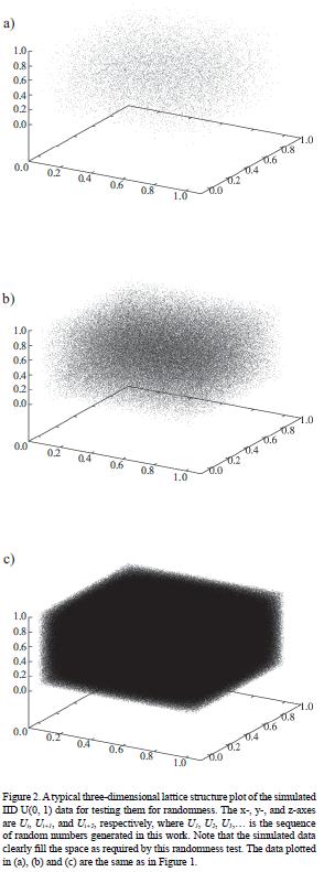
(2)  Testing of the random numbers if they resemble independent and identically distributed IID U(0, 1) random variates: Each stream was tested for randomness using Marsaglia (1968) two– and three–dimensional plot method (see also Law and Kelton, 2000, for more details). Two– and three–dimensional typical plots are shown in Figures 1 and 2, respectively. The simulated data clearly fill the (0,1) space as required by this randomness test in both two– (Figure 1 a–c for 10,000, 100,000, and 10,000,000 random numbers, respectively) and three–dimensions (Figure 2 a–c). Another test for randomness was also applied, which checks how many individual numbers are actually repeated in a given stream of random numbers, and if such repeat–numbers are few, the simulated random numbers can be safely used for further applications. On the average, only around 1 number out of 100,000 numbers in individual streams of IID U(0, 1) was repeated. Between two streams the repeat–numbers were on the average around 3 in 200,000 combined numbers, amounting to about 150 in the combined total of 10,000,000 numbers for two streams. Thus, because the repeat–numbers were so few, all 20 streams were considered appropriate for further work.

(3)  Converting the random numbers to continuous random variatesfor a normal distribution N(0, 1): The polar method of Marsaglia and Bray (1964) was employed instead of the somewhat slower trigonometric method of Box and Muller (1958). Further, this polar method was found to be sufficiently fast for our simulations and, therefore, we did not investigate any other faster scheme such as the algorithm proposed by Kinderman and Ramage (1976). Two parallel streams of random numbers (R₁j and R₂) were used for generating one set of IID N(0,1) normal random variates. Thus, from 20 different streams of IID U(0, 1), 10 sets of N(0, 1) were obtained, each one of the size 10,000,000. These simulated data were graphically examined for normality. A typical density function graph (by converting the simulated data N(0, 1) to this function using the well–known conversion equation; see Law and Kelton, 2000 or Verma, 2005 for details) is shown in Figure 3, where the data seem to approximate a normal distribution (Gaussian) curve extremely well. The "imperfections" towards the beginning [(x–µ) < –5] and end [(x–µ) > +5] of the density curve (Figure 3) are expected (see Verma, 2005 for more details) for the sample size of 10,000,000 to represent the density function (–∞ to +∞). Practically no repeat–numbers were found in tests with 100,000 numbers in these sets of random normal variates. Therefore, the data were considered of a high quality to represent a normal distribution and could, therefore, be safely used for further applications.

(4)  Computing test statistics from random normal samples of sizes up to 100: From each of these 10 sets of IID N(0, 1), random samples of sizes from 3 to 100 were drawn sequentially from each set of N(0,1) and test statistics for all 6 tests (TN7 and TN9–TN13; Table 1) were computed for each of these 10 sets of random normal variates. Thus, 10 sets of 100,000 test statistics for each value of n from 3 (for test N7) or 4 (for tests N9 and N11) or 5 (for tests N10 and N12) or 6 (for N13) to 100 were generated.

(5) Inferring critical values and evaluating their reliability: Critical values (percentage points) were computed for each of the 10 sets of 100,000 simulated test statistic values for sample sizes from 3, or 4, or 5, or 6 (depending on the type of test statistic) to 100 for all six discordance tests (N7 and N9–N13) and for different values of a from 0.30 to 0.005. By maintaining the number of individual test statistic values constant (100,000) irrespective of the size of the samples (from 3 to 100), we wanted to simulate critical values with similar standard errors of the mean for the entire set of n up to 100. This procedure was accomplished for each formula (Table 1), obtaining 100,000 test statistics for each of the 10 independent simulated sets of univariate normal samples. Thus, for test N7 (with only one test statistic formula; Table 1) only 10 such sets were generated, whereas for all other discordance tests (N9–N13), 20 sets of critical values were generated (10 sets for each formula given in Table 1). The final overall mean and median (central tendency) as well as standard deviation and standard error of the mean (dispersion) parameters were computed from 10 sets of values for test N7 and from 20 sets for tests N9–N13.

 

RESULTS OF NEW CRITICAL VALUES FOR TESTS N7 AND N9–N13

The new critical values for discordance tests N7 and N9–N13, for n from 3 up to 100 and a = 0.30 to 0.005 (corresponding to confidence levels of 70% to 99.5% or significance level of 30% to 0.5%) are summarized in Tables 2–7. (Tables 1, 2, 3, 4, 5, 6 and 7). These new critical value data (Tables 2–7), along with their uncertainty estimates, are available in other formats suchas txt or Excel or Statistica, on request from any of the authors (S.P. Verma spv@cie.unam.mx, or A. Quiroz–Ruiz aqr@cie.unam.mx).

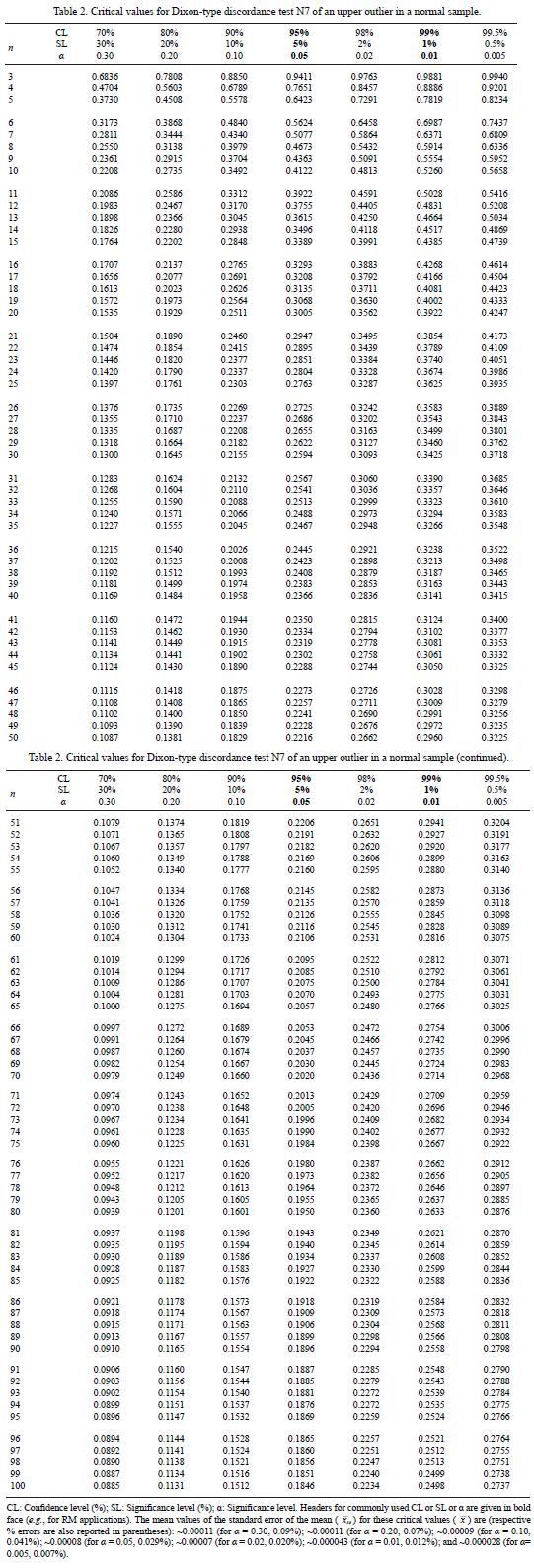
For each n (up to 100) anda (= 0.30,0.20,0.10,0.05, 0.02, 0.01, 0.005), these critical values (Tables 2–7) are the mean (x) of 10 individual simulation sets of results for testN7 and of 20 sets fortests N9–N13. It should be noted that the two formulae for a given test (N9–N13) gave very similar critical values and, therefore, these values could be combined to report single tables with more precise results (20 sets of simulations) than for test N7 (based on only 10 sets). The median critical values were found to be in close agreement with these mean values, ascertaining the simulated critical values of N7 and N9–N13 to be also normally distributed. The median values are not tabulated to limit the length of this paper and also because the sample mean for a "normal" sample appears to provide a better approximation for the central tendency than does the sample median (see e.g., Rorabacher, 1991). The standard error of the mean ( _se) was also computed and generally found to be <0.0001, irrespective of the actual value of n from 3 (or 4, or 5, or 6) to 100. The mean values of these standard errors are summarized in the footnotes of Tables 2–7 to give a clear idea of the reliability (precision and accuracy) of our new critical values (or percentage points). Thus, our present critical values are much more reliable (error is on the fourth or even on the fifth decimal place; see footnotes of Tables 2–7) than the earlier literature values quoted to only 3 decimal places (with their approximate errors 0.001–0.004 being on the third decimal place, i. e., >0.001) for n only up to 30 (Dixon, 1951; Rorabacher, 1991). In fact, this is the first time that the reliability of any set of critical values is being explicitly estimated and clearly reported; however, to limit the length of this paper, the errors available for the simulated critical values were not individually tabulated for each of the data. We also consider our new values highly accurate (accuracy being similar to the precision reported in Tables 2–7) because our simulation procedure was highly elaborated and well–tested at different stages of our work (see evaluations of simulated data in Figures 1 to 3) (Figures 1, 2 and 3) and our simulated critical values agreed to the exact values of Dixon (1951) for w = 3 and 4 to about 0.08% (see below).

Dixon (1951) presented exact solutions only for the cases where n = 3 and 4, whereas critical values for n = 5, 7, 10, 15, 20, 25, and 30 were calculated by using numerical methods; all other values for n up to 30 were estimated by interpolation with a presumed uncertainty of ± 0.001–0.004. Later, Bugner and Rutledge (1990) used a non–linear model (multi–exponential approximations of the data) to the Dixon's statistical tables. Similarly, Rorabacher (1991) used a cubic regression interpolation of Dixon's critical value data to obtain new critical values for only the so called two–sided test at the 95% confidence level; all other values were simply reproduced from Dixon (1951). Erroneous entries for test Nil corresponding to α = 0.05 in Dixon's original paper due to an upward shift of one row were, however, corrected by Rorabacher (1991).

In spite of this important observation (i.e., our simulation results being much more precise and accurate than the earlier literature values by Dixon, 1951 and Rorabacher, 1991), we decided to compare our results with the literature critical values (Figure 4) for α = 0.05 (5% SL) and 0.01 (1% SL) to find out the similarities and differences between them.

First, our present simulated critical values are characterized by very small standard errors for all values of n up to 100 (see footnotes of Tables 2–7; see also graphically the dashed and dotted near–horizontal line pairs in Figure 4a–f for n up to 100). These % errors are: 0.09% – 0.007% for test N7 (Table 2); 0.06%–0.005% for N9 (Table 3); 0.06% – 0.006% for N10 (Table 4); 0.043% – 0.014% for Nil (Table 5); 0.038%–0.014% for N12 (Table 6); and 0.037% –0.015% for N13 (Table 7). The errors of the literature critical values, on the other hand, were not really estimated by Dixon(1951) norwere stated by Barnett and Lewis (1994), but the indications are (Dixon, 1951) that they are much larger than those obtained in our present simulations (see dashed–dotted and dashed curves in Figure 4a–f, for n up to 30). Equally large errors also apply for Rorabacher (1991) critical values. Finally, due to the inaccuracies of literature critical values they differ from our present simulated values; for example, for 5% and 1% SL (Figure 4a–f), these (absolute) % differences may be as large (or even larger than) –0.4% for tests N7–N10, up to about 1.0% for test Nil (ignoring the shifted α = 0.05 values; see large circles at the lower part of the diagram in Fig. 4d), and up to about 2.0% for tests N12 and N13.

It is noteworthy that a comparison of our simulated values for n = 3 and 4 with the "exact" solutions by Dixon (1951) shows extremely small differences (mean absolute % differences of 0.08%, 0.08%, and 0.06% for tests N7, N9, and Nil, respectively), assuring thus the high accuracy of our simulated results. A part of the differences might be due to the fact that, although our values were rounded to 4 decimal places, Dixon (1951) reported these "exact" critical values to only 3 decimal places (and we do not know whether they were rounded or truncated; in any case, the report to only 3 decimal places should have caused unknown deviations from the "exact" nature of Dixon's critical values).

At first sight, from the truly statistical point of view it may appear that the more precise and accurate critical values (to 4 decimal places) such as those obtained in the present work may not represent a major advantage against the earlier less precise and accurate literature values (to 3 decimal places). Suppose we have a statistic 77V(e.g., TNT) for an observation (e.g., x_(n)), and we wish to weigh the evidence for disbelieving H₀, i.e., for judging this observation to be a discordant outlier. We assess the weight of evidence by seeing how unusual the value of T_sample is in the distribution of 77V given H₀, i.e., by P(TN>T_sample H₀) – this is the significance probability SP (T_sample), and it has a continuum of values over the range of values of T_sample – not just the familiar0.05,0.02,0.01, etc. If SP (T_sample) isvery small, say 1/500 (i.e., 0.002), the weight of evidence for disbelieving H₀ is very strong. If SP (T_sample) is quite large, say 1/5 (i.e., 0.20), the evidence for disbelieving H₀ is very weak because a 1 to 5 chance is nothing unusual. If SP (T_sample) is 0.06 or, for that matter, 0.04, there is some evidence for regarding the outlier as discordant, but it is not conclusive. If it were practicable for us to calculate the value of SP (T_sample) for our observed value (T_sample), we could assess directly the weight of evidence for rejecting H₀. But for most discordance tests, this determination of the value of SP (T_sample) is not practicable or convenient, and we make the judgment with a few "milestones": the value of (T_sample) that gives SP (T_sample) = 0.05, 0.01, or whatever. These are the tabulated critical values of 77V (Tables 2–7) such as TN7 (Table 2). Reference to these gives some indication of the weight of evidence for judging the outlier (value tested such as x_(n)) to be discordant. These are basically statistical arguments.

In practice, however, one decides a priori what value of SP (T_sample) whether 0.05 (Dybczynski, 1980; Rorabacher, 1991) or O.01 (Verma, 1997,2005), is to be used for routine operation of discordance tests. Suppose we have a value of 77V that is accurate and precise to 4 decimal places, and for which the value of SP (T_sample) for an extreme observation is 0.05025, and if we are using the criterion of 0.05 to detect discordant outliers, this observation will be detected as a discordant outlier and eliminated from the initial data set. However, suppose if we are using less precise and accurate critical values that are out by 1% as mentioned above (see Figure 4), the SP (T_sample) for the same observation happens to be 0.04975 (i.e., off by 1% with respect to 0.05025). This observation will not be detected as a discordant outlier (i. e., retained in the data set) because of our initial assumption that the value of SP (T_sample) should be greater than 0.05 set for this application, although statistically speaking both SP (T_sample) (0.05025 and 0.04975) are very similar. In other cases, the opposite action might result from the application of different sets of critical values. We, therefore, conclude that more precise and accurate critical values are preferable, if available, for all routine application of discordance tests.

 

APPLICATIONS IN SCIENCE AND ENGINEERING

In this section we present a number of examples of published data sets in science and engineering where application of these extended Dixon tests (for n up to 100) could be useful. In only some cases, the original authors reported individual experimental data. For these cases, the tests can be actually applied to provide examples of applications in science and engineering as explained below. For other cases, we can only point out how these tests will be useful. Nevertheless, we have included numerous examples from different fields of earth sciences to highlight the use of Dixon tests to actual data sets.

A spreadsheet (in Statistica commercial software) for applying these tests is available from the first author (SPV) of this paper. We may also point out that an updated version of the existing SIP VADE software (Verma et al., 1998), which will include critical values from these new tables (Tables 2–7) as well as others (under preparation), will also be made available to the scientific and industrial community for applying all discordance tests, including the six Dixon tests presented in this paper.

Rorabacher (1991), who reported new interpolated critical values for Dixon tests, argued in favor of a "two–tailed" (instead of the conventional "one–tailed") test at the 95% confidence level for such applications. We instead follow the recommendations by Verma (1997, 1998, 2005) to apply these tests "one–tailed" as is customary in such applications (see e.g., Dybczynski et al, 1979; Dybczynski, 1980; Barnett and Lewis, 1994; Verma et al., 1998; Velasco etal, 2000; Guevara et al, 2001) at the strict 99% confidence level (significance level a of 0.99) to limit the associated significance probability SP (T_sample) to 0.01 and thus have a more conclusive evidence that the outlier is discordant. Rorabacher (1991) recommendations of a "two–tailed" test would correspond to a less strict value of SP (T_sample) of 0.025 (the half of 0.05), and for this statistical reason, Verma (1997,1998,2005) proposal of using the 99% confidence level (i.e., SP (T_sample) of 0.01) would be preferable for such applications.

Dixon tests are generally used for detecting a small number of outliers, because the power of these tests decreases as the number of outliers increases in a given data set (e.g., Gibbons, 1994). Further, different kinds of masking effects make the detection of discordant outliers by a given test statistic difficult (Barnett and Lewis, 1994; Velasco et al, 2000; Buckley and Georgianna, 2001). Therefore, although in this paper we illustrate the application of Dixon tests only, the joint concurrent use of several discordance tests, such as Dixon and Grubbs tests as well as skewness and kurto–sis tests and appropriate variants of multiple–outlier tests, is highly recommended and, in fact, considered essential (Dybczynski, 1980; Verma, 1997,1998,2005; Verma et al, 1998; Velasco et al, 2000; Guevara et al, 2001).

Further work is in progress to simulate new, precise, and accurate critical values for numerous other tests summarized by Barnett and Lewis (1994) and used by Verma and collaborators in the study of geochemical reference materials. New results of this ongoing investigation we plan to publish soon in an international journal.

 

Agricultural and Soil Sciences

Stevens et al. (1995) and Lugo–Ospina et al. (2005) studied nutrients in animal manures – valuable inputs for agronomic crop production. Dixon tests can be applied to find outliers in studentized residuals (see pp. 320–323 in Barnett and Lewis, 1994, for details on such residuals) of several linear relationships used by these authors to interpret their data. In a different study, Batjes (2005) presented organic carbon data in major soil groups of Brazil, to which Dixon tests can be used to detect outliers for 13 major soil groups with the number of representative profiles from 6 to 53 (see table 2 of Batjes paper). Similarly, Luedeling et al. (2005) studied drainage, salt leaching, and physico–chemical properties of irrigated man–made terrace soils in a mountain oasis of northern Oman and used one of the Dixon tests for the evaluation of outliers. All six Dixon tests can now be better applied in such studies.

 

Aquatic Environmental Research

Thomulka and Lange (1996) studied the impact of various chemicals to aquatic environments and used a Dixon test for the evaluation of outliers. With the availability of new critical values, we suggest that all six Dixon tests be applied to such data. Similarly, Buckley and Georgianna (2001) used Dixon (1950, 1951) tests for handling statistical outliers in whole effluent toxicity data, for which new critical values of Dixon tests will be of great use.

 

Astronomy

As an example of outlier–based applications, statistical analysis of the metallicities of superclusters and moving groups by Taylor (2000) is worthy of comment. Taylor presented, in Appendix B of this paper, the use of one Dixon (1951) test for outlier detection. The new critical values derived here for all six Dixon tests would certainly facilitate the use of outlier–methods in such studies. Furthermore, for evaluating the data (in table 8 of Taylor, 2000) for the number of stars varying from 21 to 71, the author had to use a non–parametric x² test instead of the more powerful parametric tests F and Student's t (or ANOVA). With the availability of these new critical values for n up to 100, discordance tests N7 and N9–N13 can first be applied to remove any outliers and then the parametric tests (F and Student's t) can be safely applied (see Verma, 2005 for more details).

 

Biology

Linkosalo et al. (1996) and Schaber and Badeck (2002) studied tree physiology and used King (1953) test (listed as test N8 by Barnett and Lewis, 1994) for outlier detection. To the data in both papers, all Dixon tests can now be better applied than was possible earlier. For example, Schaber and Badeck (2002) presented phenological data for 9 stations (see their table 2), in which the number of observations varied from 7 to 44. Four of these stations have n > 30, for which Dixon tests, with these new critical values for n up to 100, will be now readily applicable.

 

Biomedicine and Biotechnology

Freeman et al. (1997) investigated the effects of recombinant granulocyte colony–stimulating factor during canine bacteria pneumonia. Similarly, Sevransky et al. (2005) investigated nitric oxide as a possible cause of the cardiac dysfunction associated with high, lethal doses of tumor necrosis factor–α in dogs. The number of animals in each treatment group varied from 4 to 18 in the first study and 3 to 12 in the second one. In both studies, although the authors used one of the Dixon (1950) tests, the new, precise, and accurate critical values for all six Dixon tests will render these tests to be better applicable to these data than the single Dixon test with less precise critical values. Further, even for experiments with a greater number of subjects (up to 100 in each group), Dixon tests can be now applied. Woitge et al. (1998), on the other hand, evaluated biochemical markers of bone turnover to provide information for the diagnosis and monitoring of metabolic bone disease and applied a Dixon test. All Dixon tests can now be better applied to such data.

 

Chemistry

Zaric and Niketic (1997) compiled data on Co–NO₂ bond lengths in the crystal structures of ammine–nitro complexes of cobalt(III) and applied only one outlier test (N8 by King, 1953) to these data. Neither this test nor any of the Dixon tests could have been applied to their total compiled data because the total number of data (n = 54) was much greater than 30 (being the highest n for which critical values were available). With the availability of the new critical values, all Dixon tests can now be applied to these data. The initial statistical information for Co–NO₂ bond lengths was: mean± standard deviation, 1.946 ± 0.039 Å (n = 54). After the application of Dixon tests (applied at the 95% confidence level for illustration purposes), the final statistics for the bond lengths can be summarized as: 1.938 ± 0.024 Å (n = 50).

 

Geochronology

Both Wang et al. (1998) and Dougherty–Page and Bartlett (1999) used only one test (Dixon, 1950) for outlier detection in their geochronology data. All Dixon tests with more precise and accurate critical values will be better applicable for such studies, especially when n is greater than 30. For example, Wang et al. (1998) presented Pb–Pb evaporation data (their table 3) with number of blocks up to 94, for which all Dixon tests can be applied to identify outliers. Dougherty–Page and Bartlett (1999), on the other hand, programmed a Dixon test during the data acquisition stage, for which the combination of all tests will now prove a better and more effective choice.

From the field of geochronology, we present an example from Bartlett et al. (1998) to highlight the use of Dixon tests. Single crystal zircon Pb isotopic compositions and the inferred ages were presented in their table 1 (to limit the length of this paper, the data under evaluation are not reproduced here because the reader can easily consult them in the original paper). The authors grouped the data for seven zircon grains (#1,3, 4, 6, 7, 8, and 9 in their table 1) from south India to discuss the consistency of the relevant ages (2436±11 Ma for grain #1 and 2438±12 Ma for all 7 grains; the quoted error is one standard deviation throughout this subsection). Dixon tests can now be first applied to the isotopic data of individual grains (e.g., ²⁰⁷Pb/²⁰⁴Pb data) because these experimental data should be normally distributed according to the Gauss theorem. We applied these tests to grain #1²⁰⁷Pb/²⁰⁴Pb data (n = 20) at the strict confidence level of 99% and found two lower and two upper outliers; the resulting ages can, therefore, be stated as 2435±4 Ma (n = 16). Similarly, using all (n = 33) data for the seven zircon grains and Dixon tests (at the strict confidence level of 99%), the respective age was estimated to be 2427±18 Ma (n = 31). The significantly larger dispersion of this age (±18 Ma) as compared to a single zircon grain (±4 Ma) probably reflects some age heterogeneity of the zircon grains – a characteristic not inferred by the original authors of this paper.

 

Meteorology

Graybeal et al. (2004) applied two Dixon tests (Dixon, 1950, 1951) to the seasonal and station–based analyses of hourly meteorological (temperature) data. All Dixon tests will be better applicable to this work because of more precise and accurate critical values estimated in the present study. Similarly, studentized residuals for the regressions presented by these authors can also be evaluated by these tests to detect discordant outliers.

 

Zoology

Harcourt et al. (2005) studied distribution–abundance (density) relationship of tropical mammals at the level of species, genera, and families/subfamilies. These authors eliminated outliers but their statistical method of outlier detection was not clear. Here, all Dixon tests can be easily applied to obj ectively detect outliers at the genera and family levels. Furthermore, outliers may be useful for additional geographical analysis of the data.

 

Quality assurance and assessment programs

RMs are widely used for the purpose of traceability, precision, accuracy, and sensitivity of routine analysis as well as in calibrations of analytical methods (e.g., Verma, 1997). Weighted least–squares linear regression models, instead of the conventional ordinary least–squares linear regression, are now becoming a requirement for such instrumental calibrations (e.g., Santoyo and Verma, 2003; Guevara et al., 2005). Reliable concentration (central tendency or location parameter) as well as standard deviation, standard error of the mean, or confidence limit (dispersion or scale parameter) data for each chemical constituent in the RMs are, therefore, required. However, RMs, being highly complex natural materials, are not easily prone to this type of characterization, and proper statistical methods must be applied (e.g., Barnett and Lewis, 1994; Verma, 1997,1998, 2005; Verma et al., 1998, and references therein).

Biology and Biomedicine

Ihnat (2000) evaluated the performance of neutron activation and other methods in an international reference material characterization campaign, in which the author summarized such data for large n (see table 2 of this paper). Dixon tests can now be applied to 26 sets of data, 16 of them are with n > 30; for the latter cases, Dixon tests were not earlier applicable. Similarly, Patriarca et al. (2005), in an inter–laboratory study related to their toxic metals project, used Grubbs test, among others, for the identification of outliers. Because a large number of participants (74) were involved in this study, Dixon tests can now be successfully applied to their trace element data in serum, blood, and urine samples, particularly because the new critical values are more precise and accurate than the earlier literature values.

Cement industry

Sieber et al. (2002) evaluated new cement and concrete reference materials. As an example, for Fe₂O₃ data in one reference material (SRM 1880a; see their table 5 for the inter–laboratory data; to limit the length of our paper we have not reproduced here the raw data), they reported 37 individual values, for which all Dixon tests can now be applied because of the availability of critical values for n up to 100. When Dixon tests are applied to these data at the strict confidence level of 99%, two outliers are detected in XRF data from "Construction Technology Laboratories", with the resulting statistics of mean ± standard deviation values being 2.799 ± 0.018 (n = 35). In their inter–laboratory data, Sieber et al. (2002) did not detected these outliers. The usefulness of Dixon tests is, therefore, clear from this case study, in which the application of these tests under the assumption that the data are normally distributed showed that there were two discordant outliers and, consequently, the resulting location and scale parameters will be more reliable after the application of these statistical tests.

Food science and technology

Morabito et al. (2004) and Villeneuve et al. (2004) evaluated data on organochlorinated compounds and petroleum hydrocarbons in a fish RM and methylmercury and arsenobetaine in an oyster tissue RM, respectively. Dixon tests will be readily applicable in such studies. Similarly, these tests will be useful for the food microbiology data presented by In't Veld (1998) and Langton et al. (2002).

Environmental and pollution research

Dybczynski et al. (1998), Gill et al. (2004), and Holcombe et al. (2004) analyzed inter–laboratory data for tobacco leaves, human hair, and sewage sludge RMs, respectively; it is obvious that Dixon tests with new critical values can be applied for the evaluation of these inter–laboratory data.

Nuclear science

Lin et al. (2001) evaluated radio–nuclide inter–laboratory data for the certification of RMs; in this work, the number of data varied from 18 to 84 (see table 2 of this paper). All Dixon tests with new critical values can now be applied to the data summarized by these authors.

Rock chemistry

Advantages of the availability of new critical values for Dixon tests are readily seen for several rock RMs summarized in Table 8. As an example of andesite AGV–1 from the U.S. Geological Survey, tests N7 and N9–N13, earlier applied to 0 major and 15 trace elements (Velasco–Tapia et al., 2001), can now be applied to 4 major and 39 trace elements (Table 8). In a similar way, these tests can be applied to the recently available single–laboratory raw data for Mexican RMs (Lozano and Bernal, 2005); in fact, this practice is highly recommended before estimating the location and scale parameters (see Verma, 2005 for details).

Soil science

An example of a soil RM from Peru is also listed in Table 8, for which Dixon tests, earlier applied to 5 major and 28 trace elements (Verma et al., 1998), can now be used for testing the data of 7 major and 34 trace elements.

Water research

M.P Verma (2004) compiled results of several inter–laboratory studies related to the International Association of Geochemistry and Cosmochemistry (IAGC) and International Atomic Energy Agency (IAEA), in which the number of laboratories varied from 15 to 38. Although a statistically incorrect 2s method (two standard deviation method; for more details on this method see Gladney and Roelandts, 1988a; Gladney et al., 1991; Imai et al., 1996; note that this method has been shown to be statistically incorrect by Verma, 1997, 1998) was used for outlier detection and elimination, all six Dixon tests can be readily and correctly applied to such data. Similarly, Holcombe et al. (2004) evaluated chemical data on river water, drinking water, and estuary water RMs, for which Dixon tests can now be recommended.

As a further example, we present the results of application of Dixon tests to one set of inter–laboratory HCO₃" data in water samples compiled by M.P. Verma (2004; see sample IAEA 1, n = 21, in Table 2 of the original paper), for which a mean value of 295.3 µg/ml, with a standard deviation of 18.7 µg/ml was reported. Application of all Dixon tests to these data (at the 95% confidence level, which will be the statistically correct confidence level for the erroneous "2s method") detected two upper– and two lower–outliers, obtaining the final statistics of 296 ± 9 µg/ml (n = 17).

Other Applications in Geosciences

We have already presented application of Dixon tests in geochronology and quality assurance and assessment programs in different areas of geosciences. Here, we include more areas of earth sciences to further illustrate the application of the Dixon tests using the new critical values (Tables 2–7).

Petroleum hydrocarbons and organic compounds in sediment samples

Villeneuve et al. (2002) presented such data on a sediment sample and used the Box–and–Whisker plot to detect outliers. Our Tables 2–7 enable us to apply all six Dixon tests to their data. Because of the limited availability of the report by Villeneuve et al. (2002), selected data for the illustration of these tests are summarized in Table 9. With the availability of new critical values, the Dixon tests could now be applied to the six hydrocarbon compounds in IAEA–417 compiled here. The tests (at the strict 99% confidence level) detected outlier values for 4 of the 6 hydrocarbon compounds, and the final statistics for these 4 cases showed a considerable improvement (Table 9) as compared to the original statistics on raw data. These results should be compared with the Box–and–Whisker plot method only after the application of all other discordance tests (Barnett and Lewis, 1994; Verma et al., 1998; Verma, 2005) to the data under evaluation, which will be done in future after extending the critical value tables for the remaining dozens of test variants.

Paleontology

Our first example is the LA. (índice de anchura – width index) data on Cuvieronius – one of the most common genera of the Gomphotgheriidae family recorded in Mexico during Pliocene and Pleistocene – compiled by Alberdi and Corona–M. (2005; see table 4 of this paper). Application of Dixon tests to these paleontology data did not show the presence of any outlier in these data at least with respect to the six Dixon tests and, therefore, these data can be interpreted using standard statistical techniques (outlier–based methods), although as suggested in the previous subsection, before doing so we must apply the other discordance tests to these data (work in progress).

The second example is for two different associations of ammonoids from Lower Jurassic sediments from Mexico to test the above mentioned hypotheses H₀ and H, for the diameter data of these two sets of ammonoids (see table 2 of Esquivel–Macías et al, 2005 paper). The initial statistical data were: for association 1, mean ± standard deviation 36 ± 38 (n = 35); for association 2, mean ± standard deviation 17 ± 20 (n = 59). The initial data, thus, showed a rather large variability for both associations. The Dixon tests demonstrated that each association had 2 outliers (two largest values) at the 99% confidence level, rendering the final statistics as: for association 1, mean ± standard deviation 28 ± 22 (n = 33); for association 2, mean ± standard deviation, 14 ± 9 (n = 59). The application of Dixon tests, thus, provides additional information for the interpretation of these data (see Verma, 2005 for more details).

The third example is for Maastrichtian shallow–water ammonites of northeastern Mexico to test if the WB/WH (whorl breadth to height ratio) of 16 samples (not considering "uncertain" values within brackets) reported by Ifrim et al. (2005) throughout their paper (i. e., not in a single table). The Dixon tests showed that in terms of the WB/WH variable there were no outliers in these samples, assuming that they were drawn from a normal population.

Finally, we present the fourth example from paleontology for Upper Jurassic ammonites from Sonora, Mexico (W/H data for 16 samples reported by Villaseñor et al., 2005 throughout their paper). Once again, for these ammonites the Dixon tests also showed no outliers, on the assumption that the data were drawn from a normal population.

Structural Geology

As an example of geology, we applied the Dixon tests to the inclination data of fault planes reported by Dávalos–Alvarez et al. (2005) in their Appendix C. Six inclination data sets showed a normal distribution; only for one set (FYB), one of the six Dixon tests detected outlier values.

Isotope Geology

As a further example of geology, we applied the Dixon tests to Sr isotope data on Tertiary volcanic sequences from Taxco–Quetzalapa region of southern Mexico (Morán–Zenteno et al., 1998; see nine (⁸⁷Sr–⁸⁶Sr)_i data in their table 4). According to the six Dixon tests, these data showed no outliers.

Geochemistry

As the final example for geosciences, we applied the Dixon tests to SiO₂ concentration data (100% adjusted data on an anhydrous and volatile–free basis using the SINCLAS computer program of Verma et al., 2002) of mantle–xenolith–bearing basic and ultrabasic rocks from the Eastern Alkaline Province of Mexico, recently presented by Treviño–Cázares et al. (2005). This application of the Dixon tests demonstrated that the SiO₂ concentration data assumed to come from a normal distribution in these 19 samples, showed no discordant outliers.

 

Linear regressions

This is an important area of research in almost all science and engineering fields such as for instrumental calibrations (e.g., Santoyo and Verma, 2003; Guevara et al., 2005) and for exploring relationships between two or more variables, e.g., the "inverse modeling" of trace element data (Verma, in press). Outliers in linear models can be detected and eliminated, using studentized or weighted residuals with respect to the regression equations (see pp. 315–325 in Barnett and Lewis, 1994, or pp. 40–41, 67, and 718–719 in Shoemaker et al., 1996), and the above mentioned applications of linear regressions can thus be much improved. Although Shoemaker et al. (1996) commented on the application of only one Dixon test (N7), all six tests (N7 and N9–N13) will be of much use in detecting discordant outliers in such linear models. New critical values extended to sizes of up to 100 data augment the usefulness of this approach in many more scientific and engineering problems than the ones mentioned as examples in this subsection. The new critical values for n up to 100 have paved the way for a wider application of the Dixon tests.

 

Other applications

Because of the applicability of the Dixon tests to a larger number of chemical elements (up to n= 100), it will be possible in future to use the method of Velasco etal. (2000) to empirically assess the relative efficiency of these tests by comparing their performance with that of other discordance tests. We will also be able to use the simulation procedure to assess their relative efficiency and, thus, compare the two assessments (empirical and numerical) to arrive at more definite conclusions concerning these tests.

In fact, these discordance tests (N7 and N9–N13) should be applicable to experimental data in many other scientific and engineering fields (besides the ones mentioned above), suchas ecology (Yurewicz 2004), geodesy (Kern et al., 2005), medical science and technology (Tigges et al, 1999; Hofer and Murphy 2000; Reed et al., 2002; Stancak et al., 2002), and water resources (Buckley and Georgianna, 2001).

Finally, users of a number of internet sites (e.g., San Francisco State University http://squall.sfsu.edu/courses/geo475/stats.htm; Statistics for chemists – nonparametric hypothesis tests http://www.webchem.science.ru.nl/cgi–bin/Stat/HypT/nphypt.pl; database http://www.wormbase.org; and Environmental sampling and monitoring primer http://ewr.cee.vt.edu/environmental/teach/smprimer/outlier/outlier.html) will also benefit from the incorporation of these new tables of critical values into these systems.

 

CONCLUSIONS

In synthesis, the new, precise, and accurate critical values computed for all six Dixon discordance tests offer a great advantage for diverse applications in univariate data sets, because (i) the higher precision (four significant digits instead of only three in the earlier literature values) should reduce the errors in the application of these tests because they are applied at certain significance levels of 0.05 or 0.01 in most science and engineering applications; (ii) Dixon tests (N7 and N9–N13) now have precise critical values similar to the Grubbs tests; and (iii) the increment of n up to 100 extends the application to data sets of larger sizes than was possible earlier (n was only up to 30). Finally, we must emphasize that these new critical values will open more extensive applications of these six Dixon discordance tests for normal univariate data in a variety of scientific and engineering fields, including earth sciences.

 

ACKNOWLEDGEMENTS

This research was partly supported by the "Sistema Nacional de Investigadores" (México), through a scholarship to A. Quiroz–Ruiz as the first author's (SPV's) "Ayudante de Investigador Nacional Nivel 3". The first author (SPV) is also indebted to the Editor–in–Chief Susana Alaniz–Álvarez for her kind invitation to contribute one of his papers to the journal "Revista Mexicana de Ciencias Geológicas". We are also grateful to three reviewers –who opted to remain anonymous– for providing us valuable suggestions for improvement of our earlier manuscript.

 

REFERENCES

Alberdi, M.T., Corona–M., E., 2005, Revisión de los gonofoterios en el Cenozoico tardío de México: Revista Mexicana de Ciencias Geológicas, 22(2), 246–260.        [ Links ]

Barnett, V., Lewis, T., 1994, Outliers in Statistical Data: Chichester, John Wiley, Third edition, 584 p.        [ Links ]

Bartlett, J.M., Dougherty–Page, J.S., Harris, N.B.W., Hawkesworth, C.J., Santosh, M., 1998, The application of single zircon evaporation and model Nd ages to the interpretation of polymetamorphic terrains: an example from the Proterozoic mobile belt of south India: Contributions to Mineralogy and Petrology, 131(2–3), 181–195.        [ Links ]

Batjes, N.H., 2005, Organic carbon stocks in the soils of Brazil: Soil Use and Management, 21(1), 22–24.        [ Links ]

Box, G.E.P., Muller, M.E., 1958, A note on the generation of random normal deviates: Annals of Mathematical Statistics, 29(2), 610–611.        [ Links ]

Buckley, J.A., Georgianna, T.D., 2001, Analysis of statistical outliers with application to whole effluent toxicity testing: Water Environment Research, 73(5), 575–583.        [ Links ]

Bugner, E., Rutledge, D.N., 1990, Modelling of statistical tables for outlier tests: Chemometrics and Intelligent Laboratory Systems, 9(3), 257–259.        [ Links ]

Dávalos–Álvarez, O.G., Nieto–Samaniego, A.F., Alaniz–Álvarez, S.A., Gómez–González, J.M., 2005, Las fases de deformación cenozoica en la región de Huimilpan, Querétaro, y su relación con la sismicidad local: Revista Mexicana de Ciencias Geológicas, 22(2), 129–147.        [ Links ]

Dixon, W.J., 1950, Analysis of extreme values: Annals of Mathematical Statistics, 21(4), 488–506.        [ Links ]

Dixon, W. J., 1951, Ratios involving extreme values: Annals of Mathematical Statistics, 22(1), 68–78.        [ Links ]

Dixon, W.J., 1953, Processing data for outliers: Biometrics, 9(1), 74–89.        [ Links ]

Dougherty–Page, J.S., Bartlett, J.M., 1999, New analytical procedures to increase the resolution of zircon geochronology by the evaporation technique: Chemical Geology, 153(1–4), 227–240.        [ Links ]

Dybczynski, R., 1980, Comparison of the effectiveness of various procedures for the rejection of outlying results and assigning consensus values in interlaboratory programs involving determination of trace elements or radionuclides: Analytica Chimica Acta, 117(1), 53–70.        [ Links ]

Dybczynski, R., Tugsavul, A., Suschny, O., 1979, Soil–5, a new IAEA certified reference material for trace element determinations: Geostandards Newsletter, 3(1), 61–87.        [ Links ]

Dybczynski, R., Polkowska–Motrenko, H., Samczynski, Z., Szopa, Z., 1998, Virginia tobacco leaves (CTA–VTL–2) – new Polish CRM for inorganic trace analysis including microanalysis: Fresenius Journal of Analytical Chemistry, 360(3–4), 384–387.        [ Links ]

Ebdon, D., 1988, Statistics in Geography: Oxford, Basic Blackwell, 232 p.        [ Links ]

Esquivel–Macías C., León–Olvera, R.G., Flores–Castro, K., 2005, Caracterización de una nueva localidad fosilífera del Jurásico Inferior con crinoides y amonites en el centro–oriente de México: Revista Mexicana de Ciencias Geológicas, 22(1), 97–114.        [ Links ]

Freeman, B.D., Quezado, Z., Zeni, F, Natanson, C., Danner, R.L., Banks, S., Quezado, M., Fitz, Y., Bacher, J., Eichacker, P.Q., 1997, rG–CSF reduces endotoxemia and improves survival during E–coli pneumonia: Journal of Applied Physiology, 83(5), 1467–1475.         [ Links ]

Gawlowski, J., Bartulewicz, J., Gierczak, T., Niedzielski, J., 1998, Tests for outliers; a Monte Carlo evaluation of the error of first type: Chemia Analityczna (Warshaw) Chemical Analysis, 43(4), 743–753.        [ Links ]

Gibbons, R.D., 1994, Statistical Methods for Groundwater Monitoring: New York, John Wiley, 279 p.        [ Links ]

Gill, U., Covaci, A., Ryan, J.J., Emond, A., 2004, Determination of persistent organohelogenated pollutants in human hair reference material (BCR 397); an interlaboratory study: Analytical and Bioanalytical Chemistry, 380(7–8), 924–929.        [ Links ]

Gladney, E.S., Roelandts, I., 1988a, 1987 compilation of elemental concentration data for USGS BIR–1, DNC–1 and W–2: Geostandards Newsletter, 12(1), 63–118.        [ Links ]

Gladney, E.S., Roelandts, I., 1988b, 1987 compilation of elemental concentration data for USGS BHVO–1, MAG–1, QLO–1, RGM–1, SCo–1, SDC–1, SGR–1, and STM–1: Geostandards Newsletter, 12(2), 253–262.        [ Links ]

Gladney, E.S., Jones, E.A., Nickell, E.J., Roelandts, I., 1991, 1988 compilation of elemental concentration data for USGS DTS–1, G–1, PCC–1, and W–1: Geostandards Newsletter, 15(2), 199–396.        [ Links ]

Gladney, E.S., Jones, E.A., Nickell, E.J., Roelandts, I., 1992, 1988 compilation of elemental concentration data for USGS AGV–1, GSP–1 and G–2: Geostandards Newsletter, 16(2), 111–300.        [ Links ]

Govindaraju, K., Potts, P.J., Webb, P.C., Watson, J.S., 1994, 1994 Report on Whin sill dolerite WS–E from England and Pitscurrie micro–gabbro PM–S from Scotland; assessment by one hundred and four international laboratories: Geostandards Newsletter, 18(2), 211–300.        [ Links ]

Govindaraju, K., Potts, P.J., Webb, P.C., Watson, J.S., 1995, Correction to "1994 Report on Whin sill dolerite WS–E from England and Pitscurrie microgabbro PM–S from Scotland; assessment by one hundred and four international laboratories": Geostandards Newsletter, 19(1), 97.        [ Links ]

Graybeal, D.Y., DeGaetano, A.T., Eggleston, K.L., 2004, Improved quality assurance for historical hourly temperature and humidity; development and application to environmental analysis: Journal of Applied Meteorology, 43(11), 1722–1735.        [ Links ]

Grubbs, F.E., Beck, G., 1972, Extension of sample sizes and percentage points for significance tests of outlying observations: Technometrics, 14(4), 847–854.        [ Links ]

Guevara, M., Verma, S.P, Velasco–Tapia, F., 2001, Evaluation of GSJ intrusive rocks JG1, JG2, JG3, JG1a, and JGb1: Revista Mexicana de Ciencias Geológicas, 18(1), 74–88.        [ Links ]

Guevara, M., Verma, S.P., Velasco–Tapia, F., Lozano–Santa Cruz, R., Girón, P., 2005, Comparison of linear regression models for quantitative geochemical analysis; example of X–ray fluorescence spectrometry: Geostandards and Geoanalytical Research, 29(3), 271–284.        [ Links ]

Hanson, D., Kotuby–Amacher, J., Miller, R.O., 1998, Soil analysis; Western States proficiency testing program for 1996: Fresenius Journal of Analytical Chemistry, 360(3–4), 348–350.        [ Links ]

Harcourt, A.H., Coppeto, S.A., Parks, S.A., 2005, The distribution–abundance (density) relationship; its form and causes in a tropical mammal order, Primates: Journal of Biogeography, 32(4), 565–579.        [ Links ]

Hofer, J.D., Murphy, J.R., 2000, Structured use of the median in the analytical measurement process: Journal of Pharmaceutical and Biomedical Analysis, 23(4), 671–686.        [ Links ]

Holcombe, G., Lawn, R., Sargent, M., 2004, Improvements in efficiency of production and traceability for certification of reference materials: Accreditation and Quality Assurance, 9(4–5), 198–204.        [ Links ]

Ifrim, C., Stinnesbeck, W., Schafhauser, A., 2005, Maastrichtian shallow–water ammonites of northwestern Mexico: Revista Mexicana de Ciencias Geológicas, 22(1), 48–64.        [ Links ]

Ihnat, M., 2000, Performance of NAA methods in an international interlaboratory reference material characterization campaign: Journal of Radioanalytical and Nuclear Chemistry, 245(1), 73–80.        [ Links ]

Imai, N., Terashima, S., Itoh, S., Ando, A., 1996, Database on internet for geological survey of Japan geochemical reference samples: Geostandards Newsletter, 20(2), 161–164.        [ Links ]

In't Veld, PH., 1998, The use of reference materials in quality assurance programmes in food microbiology laboratories: International Journal of Food Microbiology, 45(1), 35–41.        [ Links ]

Kern, M., Preimesberger, T., Allesch, M., Pail, R., Bouman, J., Koop, R., 2005, Outlier detection algorithms and their performance in GOCE gravity field processing: Journal of Geodesy, 78(9), 509–519.        [ Links ]

Kinderman, A.J., Ramage, J.G., 1976, Computer generation of normal random variables: Journal of American Statistical Association, 71(356), 893–896.        [ Links ]

King, E.P., 1953, On some procedures for the rejection of suspected data: Journal of American Statistical Association, 48(263), 531–533.        [ Links ]

Langton, S.D., Chevennement, R., Nagelkerke, N., Lombard, B., 2002, Analysing collaborative trials for qualitative microbiological methods; accordance and concordance: International Journal of Food Microbiology, 79(3), 175–181.        [ Links ]

Law, A.M., Kelton, W.D., 2000, Simulation Modeling and Analysis: Boston, McGraw Hill, Third edition, 760 p.        [ Links ]

Lin, Z., Inn, K.G.W., Filliben, J.J., 2001, An alternative statistical approach for interlaboratory comparison data evaluation: Journal of Radioanalytical and Nuclear Chemistry, 248(1), 163–173.        [ Links ]

Linkosalo, T., Hakkinen, R., Hari, P., 1996, Improving the reliability of a combined phenological time series by analyzing observation quality: Tree Physiology, 16(7), 661–664.        [ Links ]

Lozano, R., Bernal, J.P., 2005, Assessment of eight new geochemical reference materials for XRF major and trace element analysis: Revista Mexicana de Ciencias Geológicas, 22(3), 329–344.        [ Links ]

Luedeling, E., Nagieb, M., Wichern, F., Brandt, M., Deurer, M., Buerkert, A., 2005, Drainage, salt leaching and physico–chemical properties of irrigated man–made terrace soils in amountain oasis of northern Oman: Geoderma, 125(3–4), 273–285.        [ Links ]

Lugo–Ospina, A., Dao, T.H., Van Kessel, J.A., Reeves III, J.B., 2005, Evaluation of quick tests for phosphorus determination in dairy manures: Environmental Pollution, 135(1), 155–162.        [ Links ]

Marsaglia, G., 1968, Random numbers fall mainly in the planes: National Academy of Science Proceedings, 61(1), 25–28.        [ Links ]

Marsaglia, G., Bray, T.A., 1964, A convenient method for generating normal variables: Society for Industrial and Applied Mathematics, SIAM Review, 6(3), 260–264.        [ Links ]

Matsumoto, M., Nishimura, T., 1998, Mersenne Twister; A 623–dimensionally equidistributed uniform pseudorandom number generator: Association for Computing Machinery, ACM Transactions of Modelling and Computer Simulations, 8(1), 3–30.        [ Links ]

Morabito, R., Massanisso, P., Cámara, C., Larsson, T., Freeh, W., Kramer, K.J.M., Bianchi, M., Muntau, H., Donard, O.F.X., Lobinski, R., McSheehy, S., Pannier, F., Potin–Gautier, M., Gawlik, B.M., Bowadt, S., Quevauviller, P., 2004, Towards a new certified reference material for butyltins, methylmercury and arsenobetaine in oyster tissue: Trends in Analytical Chemistry, 23(9), 664—676.        [ Links ]

Morán–Zenteno, D.J., Alba–Aldave, L.A., Martinez–Serrano, R.G., Reyes–Salas, M.A., Corona–Esquivel, R., Angeles–García, S., 1998, Stratigraphy, geochemistry and tectonic significance of the Tertiary volcanic sequences of the Taxco–Quetzalapa region, southern Mexico: Revista Mexicana de Ciencias Geológicas, 15(2), 167–180.        [ Links ]

Muranaka, K., 1999, Teaching statistical methods: Journal of Chemical Education, 76(4), 469–69.        [ Links ]

Patriarca, M., Chiodo, E., Castelli, M., Corsetti, E., Menditto, A., 2005, Twenty years of the Me.Tos. Project; an Italian national external quality assessment scheme for trace elements in biological fluids: Microchemical Journal, 79(1–2), 337–340.        [ Links ]

Reed, D.S., Smoll, J., Gibbs, P., Little, S.F., 2002, Mapping of antibody responses to the protective antigen of Bacillus anthracis by flow cytometric analysis: Cytometry, 49(1), 1–7.        [ Links ]

Roelandts, I., 1994, Nickel and nickel alloy reference materials: Spectrochimica Acta, 49B(10), 1039–1048.        [ Links ]

Rorabacher, D.B., 1991, Statistical treatment for rejection of deviant values; critical values of Dixon's "Q" parameter and related subrange ratios at the 95% confidence level: Analytical Chemistry, 63 (2), 139–146.        [ Links ]

Santoyo, E., Verma, S.P., 2003, Determination of lanthanides in synthetic standards by reversed–phase high performance liquid chromatography with the aid of a weighted least–squares regression model; estimation of method sensitivities and detection limits: Journal of Chromatography A, 997(1–2), 171–182.        [ Links ]

Schaber, J., Badeck, F.W., 2002, Evaluation of methods for the combination of phenological time series and outlier detection: Tree Physiology, 22(14), 973–982.        [ Links ]

Sevransky, J., Vandivier, R.W., Gerstenberger, E., Correa, R., Ferantz, V., Banks, S.M., Danner, R.L., Eichacker, P.Q., Natanson, C., 2005, Prophylactic high–dose Nto–monomethyl–L–arginine prevents the late cardiac dysfunction associated with lethal tumor necrosis factor–a challenge in dogs: Shock, 23(3), 281–288.        [ Links ]

Shoemaker, D.P., Garland, C.W., Nibler, J.W., 1996, Experiments in Physical Chemistry. 6^th edition: New York, McGraw Hill, 778 p.        [ Links ]

Sieber, J., Broton, D., Fales, C., Leigh, S., MacDonald, B., Marlow, A., Nettles, S., Yen, J., 2002, Standards reference materials for cements: Cement and Concrete Research, 32(12), 1899–1906.        [ Links ]

Stancak, A., Hoechstetter, K., Tintera, J., Vrana, J., Rachmanova, R., Kralik, J., Scherg, M., 2002, Source activity in the human secondary somatosensory cortex depends on the size of corpus callosum: Brain Research, 936(1–2), 47–57.        [ Links ]

Stevens, R.J., O'Bric, C.J., Carton, O.T., 1995, Estimating nutrient content of animal slurries using electrical conductivity: Journal of Agricultural Science, 125(2), 233–238.        [ Links ]

Taylor, B.J., 2000, A statistical analysis of the metallicities of nine old superclusters and moving groups: Astronomy and Astrophysics, 362, 563–579.        [ Links ]

Thomulka, K.W., Lange, J.H., 1996, A mixture toxicity study employing combinations of tributyltin chloride, dibytyltin dichloride, and tin chloride using the marine bacterium vibrio harveyi as the test organism: Ecotoxicology and Environmental Safety, 34(1), 76–84.        [ Links ]

Tigges, M., Iuvone, P.M., Fernández, A., Sugrue, M.F., Mallorga, P.J., Laties, A.M., Stone, R.A., 1999, Effects of muscarinic cholinergic receptor antagonists on postnatal eye growth of rhesus monkeys: Optometry and Vision Science, 76(6), 397–407.        [ Links ]

Treviño–Cázares, A., Ramírez–Fernández, J.A., Velasco–Tapia, F., Rodríguez–Saavedra, P., 2005, Mantle xenoliths and their host magmas in the Eastern Alkaline Province (NE Mexico): International Geology Review, 47(12), 1260–1286.        [ Links ]

Velasco, F., Verma, S.P., Guevara, M., 2000, Comparison of the performance of fourteen statistical tests for detection of outlying values in geochemical reference material databases: Mathematical Geology, 32(4), 439–464.        [ Links ]

Velasco–Tapia, F., Guevara, M., Verma, S.P., 2001, Evaluation of concentration data in geochemical reference materials: Chemie der Erde, 61(1), 69–91.        [ Links ]

Verma, M.P., 2004, A revised analytical method for HCO₃ and CO₃²– determinations in geothermal waters; an assessment of IAGC and IAEA interlaboratory comparisons: Geostandards and Geoanalytical Research, 28(3), 391–409.        [ Links ]

Verma, S.P., 1997, Sixteen statistical tests for outlier detection and rejection in evaluation of International Geochemical Reference Materials; example of microgabbro PM–S: Geostandards Newsletter, Journal of Geostandards and Geoanalysis, 21(1), 59–75.        [ Links ]

Verma, S.P., 1998, Improved concentration data in two international geochemical reference materials, USGS basalt BIR–1 and GSJ peridotite JP–1) by outlier rejection: Geofísica Internacional, 37(3), 215–250.        [ Links ]

Verma, S.P., 2005, Estadística Básica para el Manejo de Datos Experimentales; Aplicación en la Geoquímica (Geoquimiometría): México, D.F., Universidad Nacional Autónoma de México, 186 p.        [ Links ]

Verma, S.P., in press, Extension–related origin of magmas from a garnet–bearing source in the Los Tuxtlas volcanic field, Mexico: International Journal of Earth Sciences (Geologische Rundschau).        [ Links ]

Verma, S.P., Orduña–Galván, L.J., Guevara, M., 1998, SIPVADE, A new computer programme with seventeen statistical tests for outlier detection in evaluation of international geochemical reference materials and its application to Whin Sill dolerite WS–E from England and Soil–5 from Peru: Geostandards Newsletter: Journal of Geostandards and Geoanalysis, 22(2), 209–234.        [ Links ]

Verma, S.P., Torres–Alvarado, I.S., Sotelo–Rodríguez, Z.T., 2002, SINCLAS; standard igneous norm and volcanic rock classification system: Computers & Geosciences, 28(5), 711–715.        [ Links ]

Villaseñor, A.B., González–León, C.M., Lawton, T.E., Aberhan, M., 2005, Upper Jurassic ammonites and bivalves from Cucurpe Formation, Sonora (Mexico): Revista Mexicana de Ciencias Geológicas, 22(1), 65–87.        [ Links ]

Villeneuve, J.–P, de Mora, S.J., Cattini, C., 2002, World–wide and regional intercomparison for the determination of organochlorine compounds and petroleum hydrocarbons in sediment sample IAEA–417: Vienna, Austria, Analytical Quality Control Services, International Atomic Energy Agency, 136 p.        [ Links ]

Villeneuve, J.–P., de Mora, S., Cattini, C., 2004, Determination of organo–chlorinated compounds and petroleum in fish–homogenate sample IAEA–406: results from a worldwide interlaboratory study: Trends in Analytical Chemistry, 23(7), 501–510.        [ Links ]

Wang, X.–D., Soderlund, U., Lindh, A., Johansson, L., 1998, U–Pb and Sm–Nd dating of high–pressure granulite– and upper amphibolite facies rocks from SW Sweden: Precambrian Research, 92(4), 319–339.        [ Links ]

Woitge, H.W., Scheidt–Nave, C., Kissling, C. Leidig–Bruckner, G., Meyer, K., Grauer, A., Scharla, S.H., Ziegler, R., Seibel, M.J., 1998, Seasonal variation of biochemical indexes of bone turnover: Results of a population–based study: Journal of Clinical and Endocrinological Metabolism, 83(1), 68–75.        [ Links ]

Yurewicz, K.L., 2004, A growth/mortality trade–off in larval salamanders and the coexistence of intraguild predators and prey: Oecologia, 138(1), 102–111.        [ Links ]

Zaric, S., Niketic, S.R., 1997, The anisotropic π–effect of the nitro group in ammine–nitro cobalt (III) complexes: Polyhedron, 16(20), 3565–3569.        [ Links ]