


Servicios Personalizados
Revista
Articulo
 Inglés (pdf)
 Artículo en XML
 Referencias del artículo
 Enviar artículo por email
Indicadores
-
 Citado por SciELO
 -
 Accesos
Links relacionados
-
 Similares en
SciELO
Similares en
SciELO
Compartir

 Permalink
Boletín de la Sociedad Botánica de México
versión impresa ISSN 0366-2128
Bol. Soc. Bot. Méx no.85 México dic. 2009
Ecología
Multivariate analysis of vegetation of the salted lower–Cheliff plain, Algeria
Análisis multivariado de la vegetación de la planicie salina del bajo Cheliff, Argelia
Adda Ababou1,5, Mohammed Chouieb2, Mohammed Khader3, Khalladi Mederbal3, Djamel Saidi4 and Zineddine Bentayeb4
1 Department of Biology, Faculty of Biology and Agronomy, University Hassiba Ben Bouali, Chlef, Algeria. 5 Corresponding author. E–mail: ab_adda@yahoo.fr
2 Department of Agronomy, Faculty of Science and engineering, University Abd El Hamid Ibn Badis, Mostaganem, Algeria.
3 Department of Biology, Faculty of Science and earth Sciences, University Mustapha Stambouli, Mascara, Algeria.
4 Department of Agronomy, Faculty of Biology and Agronomy, University Hassiba Ben Bouali, Chlef, Algeria
Received: april 15, 2009.
Accepted: september 23, 2009.
Abstract
The main objectives of this study were to identify the edaphic factors that could be related to vegetation distribution in the lower–Cheliff plain (35.750° – 36.125°N, 0.5° – 1°E) one the largest salted plains of northwestern Algeria and to establish the relationships between these soil factors and the main plant communities. Soil and vegetation data were obtained from 133 relevés. Species in Chenopodiaceae and Asteraceae were dominant in the salted plain. Soil variables measured included electrical conductivity, elevation, soil texture, soil structure, organic matter, CaCO3, pH, Ca++, Na+, Cl–, CaMg and color of soil. Multivariate analyses including detrended correspondence analysis (DCA) and redundancy analysis (RDA) were performed to analyze the collected data. The results showed that the vegetation distribution pattern was mainly related to conductivity and elevation. Separation of relevés into groups according to the first two axes of RDA provided four vegetation units, each one composed of several diagnostic species with highly significant fidelity value according to Fisher's test. The theoretical maps produced by kriging revealed a close relationship between these vegetation units and conductivity.
Key words: Redundancy analysis, vegetation units, salinity, cartography, lower–Cheliff, Algeria.
Resumen
El objetivo de este trabajo es identificar los factores edáficos que tienen un efecto en la distribución de la vegetación en la planicie del bajo Cheliff (35.750° – 36.125°N, 0.5° – 1°E), una de las zonas salinas más grandes del noroeste de Algeria y asimismo establecer las relaciones entre estos factores del suelo y la distribución de las comunidades vegetales. Para cumplir con este objetivo se muestreó la vegetación y el suelo de 133 relevés. Las familias con un mayor número de especies dominantes fueron las Chenopodiaceae y Asteraceae. Las variables edáficas medidas incluyeron la conductividad electríca, la textura, la estructura, materia orgánica, CaCO3, pH, Ca++, Na+, Cl–, CaMg y el color de los suelos. Además se tomó en cuenta la elevación. Los datos se analizaron por métodos multivariados incluyendo el análisis de correspondencia de residuales (DCA por sus siglas en inglés) y el análisis de redundancia (RDA por sus siglas en inglés). Los resultados mostraron que el patrón de distribución de la vegetación estuvo relacionado sobre todo a la conductividad del suelo y a la elevación. La separación de relevés en grupos de acuerdo a los dos ejes del análisis de redundancia fueron en cuatro unidades de vegetación, cada una compuesta por varias especies diagnósticas con un alto valor de fidelidad de acuerdo a la prueba de Fisher. Los mapas elaborados corroboraron que existe una clara relación entre las unidades de vegetación y la conductividad del suelo.
Palabras clave: Análisis de redundancia, unidades de vegetación, salinidad, cartografía, bajo Cheliff Algeria.
For over a century, ecologists have attempted to determine the factors that control plant species distribution and variation in vegetation composition (Motzkin et al., 2002). Indeed in order to better understand and manage the stressed ecosystems, it is important to study the relationship between environmental factors and plants. One of the main components of these ecosystems is vegetation, the absence and presence of which is controlled by environmental variables such as soil, topography and climate (Cook and Irwin, 1992; Jafari et al., 2004). Among different environmental factors, soil is of high importance in plant occurrence, and it is a function of climate, organisms, topography, parent material and time (Hoveizeh, 1997). Effects of environmental factors on plant communities have been the subject of many ecological studies in recent years, much of the research on species–environment relationships has been carried out in semiarid regions of North America, Australia, and other desertic regions, such as Egypt, India, Iran, etc. (Moreno–Casasola and Espejel, 1986; Parker, 1991; Castillo, Popma and Moreno–Casasola, 1991; Comstock and Ehleringer, 1992; Abd El–Ghani and Amer, 2003; Amiri and Saadatfar, 2009). Our knowledge about interactions of the vegetation distribution and environmental factors in semi arid regions of Algeria is rather poor. Determining which factors influence occurrence and relative abundance of plant species remains a central goal of research in arid and semi–arid ecosystems. The lower–Cheliff plain one of the largest alluvial plains of northwestern Algeria belonging to semi–arid ecosystems is the homeland of diverse plant species.
For analyzing the relationship of species occurrence to site conditions in the lower–Cheliff plain, some direct gradient analyses could be useful, either a redundancy analysis (RDA) or a canonical correspondence analysis (CCA) (Leps and Smilauer, 2003; Zuur et al., 2007). Also statistical fidelity measures (Chytry et al., 2002) such as Φ–coefficient can be employed to characterize the floristic composition of a given site, independently of environmental conditions. In this context, the main purpose of this research was: (1) to determine which plant species inhabit the lower–Cheliff plain. (2) to perform a redundancy analysis (RDA) to determine the topographic and edaphic factors that influence plant species occurrence to understand the most important components affecting the segregation of plant species. (3) to analyze the vegetation assemblage independently to the site conditions by calculating the Φ–coefficient of association in order to extract the main vegetation units and compare the vegetation units oppossed to the strongest environmental factors affecting the lower–Cheliff.
Understanding relationships between ecological variables and plant species in this ecosystem helps us to map out the different vegetation units in the lower–Cheliff, in order to apply these findings in management and development of this region.
Material and methods
Study area. Covering approximately 450 km2 the lower–Cheliff is one of the largest Quaternary alluvial plains of northwestern Algeria (figure 1). This region, located between 35.750° – 36.125°N of latitude and 0.5° –1°E of longitude, is about 35 km inland from the Mediterranean Sea, with an average altitude of 70 m. The plain is a syncline framed on the north by the Dahra hills and the Benziane hills on the South both characterized by clayey silt, schist and salted marls (MC Donald and B.N.D.E.R, 1990). These geological characteristics, accentuated by a semi–arid climate with an average annual temperature of 20° C and a weak annual pluviometry (approximately 250 mm/yr), explain the high salinity conditions of the plain. Soil and vegetation sampling. Vegetation relevés were recorded during spring 2006, 2007 and 2008 (March 21st – May 21st) by using the Braun–Blanquet (van der Maarel, 1975) seven–point scale of abundance–dominance then transformed to 0–9 van der Maarel scale. A total of 133 relevés were recorded adding up 40 species among which 11 were rare species that were excluded from the analysis. Also, a total of 133 soil samples were collected at a depth of 30 cm. Measured soil factors were physical (granulometry, soil structure (S.S), ground colors (RGB)), chemical (conductivity (ECe), CaCO3, pH, Ca++, Na+, Cl–, organic matter (o.M) and CaMg) and topographical nature (elevation). in order to use geostatistical analysis the geographical position of each site was determined by using GPS. Data analysis. Initially, a co–linearity test performed between environmental variables showed a strong correlation coefficient (R > 0.9) between sands and silt, Na+ and Cl–. Therefore, we chose to eliminate Cl– and silt. Then, the remaining variables were subjected to a Shapiro–Wilk's normality test; those with non–normal distribution were log–transformed. For determination of the most significant variables an individual pre–selection (Okland and Eilertsen, 1994) was performed by using a Monte Carlo test (999 permutations without restriction), with the exception of sand, they were all significant (P < 0.05) with variance inflation factors (Chatterjee and Price, 1991 ; Erkel–Rousse, 1995; Besse, 2001; O'brien, 2007) < 4 indicating no colinearity. (table 1).
In order to establish the main links between environmental variables and vegetation assemblage, a redundancy analysis (RDA) (ter Braak, 1994; Legendre and Legendre, 1998; Skinner et al., 1998; Leps and Smilauer, 2003) was performed. First, a detrended correspondence analysis (DCA) (Hill and Gauch, 1980) was conducted in order to decide whether a model with unimodal (CCA) (ter Braak, 1986) or linear (RDA) response curve should be used in ordination analysis. Results of the DCA showed that gradient length was 3.95 for axis 1 to 2.53 for axis 4; thus, both RDA and CCA may give correct results (Leps and Smilauer, 2003; Jongman et al., 1996). As the percentage of total variance explained by RDA (21%) was higher than CCA (17.2%), we considered it more appropriate to perform an RDA, as linear relationships between species and environmental variables. However the presence of double zeros strongly affects the RDA with another potential problem, namely the arch effect (Zuur et al., 2007). An alternative is to apply either chord (Orloci, 1967) or Hellinger (Rao, 1995) distances transformation. Legendre and Gallagher (2001) showed that this approach is less sensitive to double zeros and consequently to the arch effect. After several comparisons, we chose the Hellinger transformation followed by an RDA. The most significant variables were determined by using the method Wilk's lambda (Butler and Wood, 2004; Marques de Sa, 2007).
To cluster samples into similar groups and to identify the characteristic vegetation unit of each group, relevés were separated into groups, according to their coordinates based on the first two canonical axes obtained by RDA. Finally, four pre–defined groups were used because they showed major ecological relevance and were easily interpretable. We used the Φ–coefficient of association (Sokal and Rohlf, 1995; Chytry et al., 2002) to identify species discriminating between the four groups. This coefficient is a statistical measure of association which can be used as a measure of fidelity, and it can be calculated as follows:
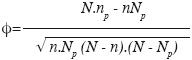
We used in this study the same notation as in Bruelheide, (2000) and Chytry et al., (2002): N = number of relevés in the data set Np = number of relevés in the particular vegetation unit; n = number of occurrences of the species in the data set; and np = number of occurrences of the species in the particular vegetation unit.
Traditionally, the Φ–coefficient considers only the presence/absence (binary) information for the species, so that fidelity values calculated using this coefficient are not influenced by species cover or abundance. The advantage of the Φ–coefficient is its independence of dataset size. The Φ–coefficient ranges from –1 to 1. The highest Φ value (1) is achieved if the species occurs in all relevés of the vegetation unit and is absent elsewhere. A positive value but lower than 1 implies that the species is absent from some relevés of the vegetation unit. A value of 0 indicates no relation between the target species and the target vegetation unit.
Finally, in order to establish the relation between vegetation and salinity a map was constructed out using Krig–ing (Krige, 1951; Journel and Huijbregts, 1978; Stein et al., 2002).
Results and discussion
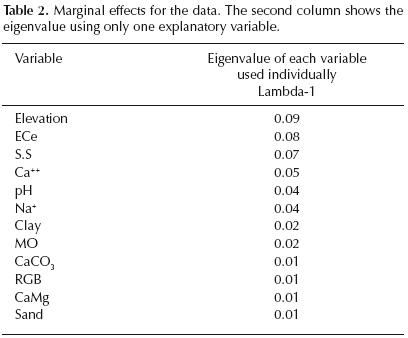
Variables ranking. The marginal effects showing the eigenvalue of explained variance if only one explanatory variable is used in RDA (table 2) indicate that elevation, conductivity and soil structure are the best explanatory variables, followed by Ca++, pH, and Na+, whereas the remaining variables play a secondary role.
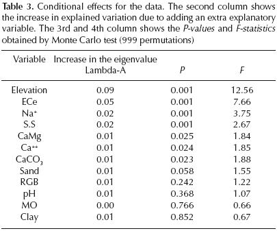
The highly significant (P < 0.01) increases in the total sum of eigenvalues during the forward selection indicated by the conditional effects (table 3) are shown successively by elevation, conductivity, Na+ and soil structure, according to Monte Carlo test (999 permutations). CaCO3, Ca++ and CaMg confered significant increases (P < 0.05), whereas the contribution of the remaining variables were not significant. Best predictors of plant species distribution. The variance of species occurrence data explained by each variable according to the partial RDA is in the following order: elevation = 8.8%, conductivity = 7.7%, soil structure = 6.5%, Ca++ = 4.6%, pH = 4.5%, Na+ = 3.5%, Clay = 2.3%, OM = 1.7%, CaCO3 = 1.4%, RGB=1.4%, CaMg = 1.2% and Sand = 0.9%. This means that the distribution of species in the lower–Cheliff plain is strongly correlated to elevation, conductivity and soil structure.
Redundancy analysis. The ordination analysis (table 4) showed a strong environmental gradient in the area. The lengths of gradient, retrieved by DCA, were 3.95 on the first axis to 2.53 on the fourth. The RDA showed a low cumulative percentage variance of species occurrence data explained on the first four axes of the RDA (21.0%) (table 4). However, there was a strong relationship between the vegetation and the environmental factors, with species–environment correlations of 0.82 on the first axis and 0.68 on the second. Although the Monte Carlo permutation test indicates that all canonical axes were highly significantly correlated with the set of variables used, only the first two canonical axes were used because they included the maximum variability expressed by the environmental variables (71.8% of the variance of species–environment relationship), and almost all variables that were significant on axes 3 and 4 were also significant on axes 1 and 2. The first axis explained almost 55% of the variance of species–environment relationship, this axis is mainly negatively correlated to conductivity, and then to Ca++, Na+ and clay, while it is positively correlated mainly with elevation, and subsequently to soil structure, pH, organic matter and CaCO3. This means that sampling sites situated on the right side of the first axis are characterized by higher elevations, and low conductivity. On the left side of this axis sampling sites with higher conductivities are shown. Thus, axis 1 represents a gradient of decreasing elevations and increasing conductivities and thus salinity. This axis could be interpreted as conductivity environmental gradient. Low elevations are accompanied by salts deposits exacerbated by a high proportion of clay, which prevents salts drainage. This process leads to high conductivity and the degradation of soil structure, indeed according to Papatheodorou (2008), the main influence of salt in soil is the dispersion of clay particles with consequent changes in soil physicochemical properties. With appearance of halophilous species such as those in the Chenopodiaceae and Caryophyllaceae, characteristic of the extreme salinity conditions (figure 2). Relative high elevations characterized by low conductivity and a slightly high organic matter rate, which improves the soil structure and allows a more diversified floristic composition (Asteraceae, Fabaceae, Geraniaceae, Apiaceae, Brassicaceae, Primulaceae, Plantaginaceae).
The second axis with 16.8% of the variance of species–environment relationship explained is negatively correlated with RGB, pH and sand, and positively correlated mainly with conductivity and Na+, with a notable occurrence of Chenopodiaceae and Caryophyllaceae. As a result it is clear that in the study area, among different environmental factors (topographic and edaphic variables), the distribution of vegetation was most strongly correlated to conductivity. Indeed this observation was reported by many investigators (Ungar, 1968; Zahran et al., 1989; Caballero et al., 1994; Maryam et al., 1995; Alvarez–Rogel et al., 2000; Trites and Bayley, 2009) who studied the relation between species distribution and salinity gradient.
Vegetation units according to fidelity coefficient. The plant association is "a plant community characterized by definite floristic and sociological features" that shows, by the presence of diagnostic species "a certain independence" (Braun–Blanquet, 1928) and grows under uniform habitat conditions (Flahault and Schroter, 1910). These plant communities are generally recognized by diagnostic species as defined by Westhoff and van der Maarel, (1973). In this context, the concept of diagnostic species is important in vegetation classification; it is a plant of high fidelity to a particular community that serves as a criterion of recognition of that community (Curtis, 1959). The relative constancy or abundance of diagnostic species allows to distinguish one association from another (Whittaker, 1962; Chytry and Tichy, 2003). One plant association includes species that preferably occur in a single vegetation unit (character species) or in a few vegetation units (differential species) (Chytry et al., 2002). Their presence, abundance, or vigor are considered to indicate certain site conditions (Gabriel and Talbot, 1984).
The two first canonical axes were used in the classification of sites cluster to all samples, because they include the maximum variability expressed by environmental variables. As a result, four distinct groups of sites with similar floris–tic composition were identified. Group A comprised 43 sites characterized by the lowest elevations and salty grounds. These sites were differentiated by the presence of six diagnostic species, on the basis of the results of the Φ–coefficient; the most significant species are Plantago coronopus and Bellis perennis (Table 5). Diagnostic species present in this group as indicated by the distribution curve (figure 3a) were generally associated to salty grounds. Group B included 25 sites with the highest elevations and the lowest conductivity, it was characterized by four diagnostic species very sensitive to salinity as indicated by distribution curve (figure 3b). Group C with the highest diversity according to the Shannon index (table 5), was composed of 30 slightly salty sites, intermediate elevations and characterized by eight diagnostic species including Sinapis arvensis, Plantago lanceolata and Scolymus hispanicus with the highest fidelity to this group. The distribution curve (figure 3c) shows that diagnostics species of this group were associated with the lowest salinity. Finally, group D included 35 sites highly salty; the five diagnostic species of this group exclusively belong to Chenopodiaceae and Caryophyllaceae. As shown by the distribution curve (figure 3d) the presence of diagnostic species of this group indicate highly salty grounds. Groups A and D were the less diverse groups according to Shannon index (table 5), this low diversity is caused by the high salinity of these two groups of sites. It is because salt at higher concentrations in apoplast of cells generates primary and secondary effects that negatively affect survival, growth and development. Primary effects are ionic toxicity, disequilibrium, hyperosmolality and hyperosmotic shock. Principal secondary effects of salt stress include disturbance of K+ acquisition, membrane dysfunction, impairment of photosynthesis and other biochemical processes, generation of reactive oxygen species and programmed cell death (Botella et al., 2005). Low diversity in these two groups is an evidence of salty material. Only high adaptability plants to salinity can grow in these conditions. According to Zhu (2003), plants that are native to saline environments (halo–phytes) use many conserved cellular and organismal processes to tolerate salt. This salt tolerance is related to genetic adaptations (Munns, 2002; Flowers, 2004). To avoid salinity stress, they have developed a very effective mechanism for selective cation uptake. They evidently posses potassium transporters with no or only very little affinity for sodium, and are thus able to exclude Na+ from their tissues. Other halophytes with a less selective K+ uptake system make use of the fact that Na+ and Cl– are phloem–mobile ions which are able to circulate within the plant. They accumulate salt at the base of the stem, while the growing parts of the plant are kept largely salt free (Schulze et al., 2005). Whereas according to Gurevitch et al. (2006), osmoregulation is particularly important in allowing many halophytes growing in saline soils (where soil water has a negative water potential largely due to a negative osmotic potential caused by dissolved salts) to maintain a favorable water potential gradient. Other halophytes have the ability to excrete salt.
Thus, results demonstrate that there is a specific relationship between soil characteristics and the separation of the plant species. Soil salinity and its variation is the main factor that causes separation of the plant species in the study area.
As shown by the RDA (figure 2) and distribution curves (figure 3), diagnostic species of vegetation A and especially unit D are indicators of saline lands with a fine texture soil. By contrast, diagnostic species of vegetation unit B are indicators of unsalted soils with good soil structure, while diagnostic species of vegetation unit C grow on slightly salty soils.
Electrical conductivity. All theoretical variograms used to estimate electrical conductivity show a high nugget effect, high variance and a strong variation coefficient (Table 6). Electrical conductivity is consequently an unpredictable and slightly structured variable, with a strong variability even at very short distances. This requires a high density of sampling to predict electrical conductivity.
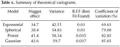
On the basis of variographic analysis (table 6) and cross validation (R2 = 0.73 and S.E.E (standard error of estimate) = 4 mmhos) (figure 4), exponential model is the best theoretical model to estimate electrical conductivity.
The estimated conductivity map (Figure 5) shows first, an increasing conductivity from East to West and from the periphery to the center of the plain. This corresponds to a decreasing elevation from East to West and from periphery to the center. Secondly, a very large surface of the lower–Cheliff plain belongs to the range of salty to highly salty grounds.
Spatial distribution of vegetation units according to conductivity. Transformation of species abundance from Braun–Blanquet scale to 0–9 van der Maarel scale enabled us to map out the spatial distribution of the vegetation units through kriging. As a result the figure 6, show a close relationship between vegetation units and electrical conductivity. Vegetation unit A (figure 6a) is distributed throughout the salty grounds according to the same gradient of salinity, from the periphery to the center and from the East to the West. Vegetation unit D (figure 6d) occupies the highly salty grounds, whereas vegetation unit B (figure 6b) is completely absent from the western side of the plain characterized by salty grounds and low elevations. Vegetation unit C (Figure 6c) is especially localized at the periphery of the plain characterized by slightly salty grounds.
Conclusion
The lower–Cheliff plain is an ecosystem stressed by particular edaphic constraints and hard climatic adversities. These constraints reduce strongly plant diversity. Thus, during three years of study, we recorded only 40 species through 133 relevés.
With an aim of a reasoned management strategy for this ecosystem, traditional methods of evaluation of site conditions are expensive and time consuming, especially in areas as large as the Lower–Cheliff; thus, recognition of vegetation ecology and biology is the easiest way of decreasing cost and saving time in the assessment of environmental conditions. The present study provides baseline information on the environmental variables affecting distribution patterns of vegetation assemblages in one of the largest plains in Algeria. it is clear that the understanding of local scale factors is needed to assess the importance of factors structuring plant communities. The key factors that determine the distribution of vegetation in the lower–Cheliff plain are elevation, conductivity, sodium and soil structure. However, according to our study one of the most important factors that influence the composition of vegetation assemblages is conductivity. Indeed, we were able to differentiate among four vegetation units in relation to the influence of this important environmental variable. We distinguished less diverse vegetation units composed of halophilous species, distributed throughout the salty grounds and more diverse vegetation units, very sensitive to salinity, occupying the unsalty to slightly salty grounds. Thus, the assessment of plant communities is a useful tool to classify salinity, especially in terms of revealing the spatio–temporal changes of this variable. it would be interesting to compare these results with other vegetation study in the same condition.
Literature cited
Abd El–Ghani M.M and Amer W.M. 2003. Soil–vegetation relationships in coastal desert plain of southern Sinai, Egypt. Journal of Arid Environments 55: 607–628. [ Links ]
Alvarez–Rogel J., Alcaraz–Ariza F. and Ortiz–Silla R. 2000. Soil salinity and moisture gradients and plant zonation in Mediterranean salt marshes of Southeast Spain. Wetlands 20:357–372. [ Links ]
Amiri F. and Saadatfar A. 2009. Using ordination method for determination of effective environmental factors on Astragalus parrawinus species establishment in semi–arid regions of Iran. Asian Journal of Plant Sciences 8:11–19. [ Links ]
Besse P 2001. Pratique de la Modélisation Statistique, Publications du Laboratoire de Statistique et Probabilité. Université Paul Sabatier. Toulouse. [ Links ]
Botella M.A., Rosado A., Bressan R.A. and Hasegawa P.M. 2005. Plant adaptive responses to salinity stress. In: Jenks M.A and Hasegawa P.M. Ed. Plant Abiotic Stress, pp. 38–70, Blackwell Publishing, India. [ Links ]
Braun–Blanquet J. 1928. Pflanzensoziologie. Grundzuge der Veg–etationskunde. Springer–Verlag, Wien. [ Links ]
Bruelheide H. 2000. A new measure of fidelity and its application to defining species groups. Journal of Vegetation Science 11:167–178. [ Links ]
Butler R.W. and Wood A.T.A. 2004. A dimensional CLT for non–central Wilk's lambda in multivariate analysis. Scandinavian Journal of Statistics 31:585–601. [ Links ]
Caballero J.M., Esteve M.A., Calvo J.F. and Pujol J.A. 1994. Structure of the vegetation of salt steppes of Guadelenitin (Murcia, Spain). Studies in Oecologia 10–11:171–183. [ Links ]
Castillo S., Popma J. and Moreno–Casasola P 1991. Coastal sand dune vegetation of Tabasco and Campeche. Journal of Vegetation Science 2:73–88. [ Links ]
Chatterjee S. and Price B. 1991. Regression Analysis by Example. John Wiley and Sons, New York. [ Links ]
Chytry M. and Tichy L. 2003. Diagnostic, constant and dominant species of vegetation classes and alliances of the Czech Republic: a statistical revision. Folia–Biologia No 108. Faculty of Sciences natural from University Masarykianae Brunensis. Brno, Czech Republic. [ Links ]
Chytry M., Tichy L., Holt J. and Botta–Dukat Z. 2002. Determination of diagnostic species with statistical fidelity measures. Journal of Vegetation Science 13:79–90. [ Links ]
Comstock J.P. and Ehleringer J.R. 1992. Plant adaptation in the Great Basin and Colorado Plateau. Great Basin Naturalist 52:195–215. [ Links ]
Cook J.G. and Irwin L.L. 1992. Climate–vegetation relationships between the Great Plains and Great Basin. American Midland Naturalist 127: 316–326. [ Links ]
Curtis J.T. 1959. The vegetation of Wisconsin. An ordination of plant communities. University of Wisconsin Press, Madison, Wisconsin. [ Links ]
Erkel–Rousse H. 1995. Détection de la multicolinéarité dans un modèle linéaire ordinaire : quelques éléments pour un usage averti des indicateurs de Belsley, Kuh et Welsh. Revue de statistique appliquée 43:19–42. [ Links ]
Flahault C. and Schroter C. 1910. Rapport sur la nomenclature phytogeographique. Proceedings of the 3rd International Botanical Congress, Brussels 1:131–164. [ Links ]
Flowers T. J. 2004. Improving crop salt tolerance. Journal of Experimental Botany 55:307–319. [ Links ]
Gabriel H.W. and Talbot S.S. 1984. Glossary of landscape and vegetation ecology for Alaska. Alaska Technical Report 10. Bureau of Land Management, Washington, D.C. [ Links ]
Gurevitch J., Scheiner S.M. and Fox G.A. 2006. The Ecology of Plants. Sinauer Associates, Inc., Sunderland. [ Links ]
Hill M.O. and Gauch H.G. 1980. Detrended correspondence analysis, an improved ordination technique. Vegetatio 42:47–58. [ Links ]
Hoveizeh H. 1997. Study of the vegetation cover and ecological characteristics in saline habitats of Hoor–e–Shadegan. Journal of Research and Construction 34:27–31. [ Links ]
Jafari M., Zare Chahoukib M.A., Tavilib A., Azarnivandb H. and Zahedi Amirib Gh. 2004. Effective environmental factors in the distribution of vegetation types in Poshtkouh rangelands of Yazd Province (Iran). Journal of Arid Environments 56: 627–641. [ Links ]
Jongman R.H.G., Ter Braak C.J.F. and van Tongeren O.F.R. 1996. Data analysis in community and landscape ecology. Cambridge University Press. Cambridge. [ Links ]
Journel A.G. and Huijbregts C.J. 1978. Mining Geostatistics. Academic Press, San Diego, CA. [ Links ]
Krige D.G. 1951. A statistical approach to some basic mine valuation problems on the Witwatersrand. Journal of the Chemical, Metallurgical and Mining Society of the South Africa 52:119139. [ Links ]
Legendre P. and Legendre L. 1998. Numerical Ecology. Elsevier. Amsterdam. [ Links ]
Legendre P. and Gallagher E. 2001. Ecologically meaningful transformation for ordination of species data. Oecologia 129:271280. [ Links ]
Lep J. and
  milauer P. 2003. Multivariate analysis of ecological data using CANOCO. Cambridge University Press. Cambridge. [ Links ]
MC Donald and B.N.E.D.E.R. 1990. Etude de l'avant projet détaillé des extensions de Guerouaou et de Sabkhat Benziane et du réaménagement du Bas Cheliff. Bureau National d'Etude pour le Développement Rural. Tome I. Etude du milieu physique 192p. [ Links ]
Maryam H., Ismail S., Alaa, F. and Ahmed R. 1995. Studies on growth and salt regulation in some halophytes as influenced by edaphic and climatic conditions. Pakistani Journal of Botany 27:151–163. [ Links ]
Marques de Sá J.P. 2007. Applied Statistics Using SPSS, STATISTICA, MATLAB and R. Springer–Verlag, Berlin Heidelberg. [ Links ]
Moreno–Casasola P. and Espejel I. 1986. Classification and ordination of coastal sand dune vegetation along the Gulf and Caribbean Sea of Mexico. Vegetatio 66:147–182. [ Links ]
Motzkin G., Eberhardt R., Hall B., Foster D. R., Harrod J. and MacDonald D. 2002. Vegetation variation across Cape Cod, Massachusetts: environmental and historical determinants. Journal of Biogeography 29:1439–1454. [ Links ]
Munns R. 2002. Comparative physiology of salt and water stress. Plant, Cell and Environment 25:239–250. [ Links ]
O'brien R.M. 2007. A caution regarding rules of thumb for variance inflation factors. Quality and Quantity 41:673–690. [ Links ]
Økland R.H. and Eilertsen O. 1994. Canonical correspondence–analysis with variation partitioning – some comments and an application. Journal of Vegetation Science 5:117–126. [ Links ]
Orloci L. 1967. An agglomerative method for classification of plant communities. Journal of Ecology 55:193–206. [ Links ]
Papatheodorou E.M. 2008. Responses of soil microbial communities to climatic and human impacts in Mediterranean regions. In: Liu, T. Soil Ecology Research Developments pp. 63–87. Nova Science Publisher, New York. [ Links ]
Parker K. 1991. Topography, substrate, and vegetation patterns in the northern Sonoran Desert. Journal of Biogeography 18:151–163. [ Links ]
Rao C.R. 1995. A review of canonical coordinates and an alternative to correspondence analysis using Hellinger distance. Questiio. 19:23–63. [ Links ]
Schulze E., Beck E. and Muller–Hohenstein K. 2005. Plant ecology. Springer, Berlin. [ Links ]
Skinner W.R., Jefferies R.L., Carleton T.J., Rockwell R.F. and Abraham K.R. 1998. Prediction of reproductive success and failure in lesser snow geese based on early season climatic variables. Global Change Biology. 4:3–16. [ Links ]
Sokal R.R. and Rohlf F.J. 1995. Biometry. The Principles and Practice of Statistics in Biological Research. W.H. Freeman and Company, New York. [ Links ]
Stein A., van der Meer F. and Gorte B. 2002. Spatial Statistics for Remote Sensing. Kluwer academic publishers, The Netherlands. [ Links ]
ter Braak C.J.F. 1986. Canonical correspondence analysis: a new eigenvector technique for multivariate direct gradient analysis. Ecology 67:1167–1179. [ Links ]
ter Braak C.J.F. 1994. Canonical community ordination. Part I: Basic theory and linear methods. Ecoscience 1:127–140. [ Links ]
Trites M. and Bayley S.E. 2009. Vegetation communities in continental boreal wetlands along a salinity gradient: Implications for oil sands mining reclamation. Aquatic Botany 91:27–39. [ Links ]
Ungar I.A. 1968. Species–soil relationships on the great salt plains of northern Oklahoma. American Midland Naturalist 80:392406. [ Links ]
van der Maarel E. 1975. The Braun–Blanquet approach in perspective. Vegetatio 30:213–219. [ Links ]
Westhoff V. and van der Maarel E. 1973. The Braun–Blanquet approach. In: Whittaker R.H. Ed. Ordination and Classification of Plant Communities pp. 617–737. Dr. W. Junk Publiser, The Hague. [ Links ]
Whittaker R.H. 1962. Classification of natural communities. The Botanical Review 28:1–239. [ Links ]
Zahran M.A., Abu Ziada M.E., El–Demerdash M.A. and Khedr A.A. 1989. A note on the vegetation on islands in lake Manzala, Egypt. Vegetation 85:83–88. [ Links ]
Zhu J.K. 2003. Regulation of ion homeostasis under salt stress. Current Opinion in Plant Biology 6:441–445. [ Links ]
Zuur A.K., Ieno E.N. and Smith G.M. Eds. 2007. Analysing Ecological Data. Springer, New York. [ Links ]

