


Servicios Personalizados
Revista
Articulo
 texto en
  Inglés (pdf)
 Artículo en XML
 Referencias del artículo
 Enviar artículo por email
Indicadores
-
 Citado por SciELO
 -
 Accesos
Links relacionados
-
 Similares en
SciELO
Similares en
SciELO
Compartir

 Permalink
Problemas del desarrollo
versión impresa ISSN 0301-7036
Prob. Des vol.54 no.214 Ciudad de México jul./sep. 2023 Epub 18-Mar-2024
https://doi.org/10.22201/iiec.20078951e.2023.214.70000
Articles
Global value chains at the bilateral-sectoral level between Texas-Mexico and California-Mexico
aEl Colegio de la Frontera Norte, Mexico. Email: afuentes@colef.mx ; davidgaytan@colef.mx and abrugues@colef.mx, respectively.
This article estimates and analyzes the value-added chains embedded in the bilateral-sectoral trade of intermediate and final goods included in the transactions: Texas-Mexico (TX-MX) and California-Mexico (CA-MX). For this purpose, the global interregional input-output matrices for TX-MX and CA-MX were constructed for 2013. The bilateral-sectoral trade balance shows that Texas (TX) and California (CA) specialize in exports of intermediate goods. In contrast, Mexico (MX) specializes in final goods, resulting in low export multipliers for the latter. MX maintains high dependence on intermediate goods from TX, CA, and third places, resulting in lower foreign exchange earnings per dollar exported. Finally, TX-MX has an energy-technology trade pattern, while CA-MX has a technology-energy trade pattern.
Keywords: global value chains; input-output model; multiregional analysis
El objetivo del presente artículo es estimar y analizar las cadenas de valor agregado incorporado en el comercio bilateral-sectorial de mercancías intermedias y finales que forman parte de las transacciones: Texas-México (TX-MX) y California-México (CA-MX). Para ello se construyeron las matrices insumo producto interregionales globales de TX-MX y CA-MX para 2013. El balance de comercio bilateral-sectorial muestra que Texas (TX) y California (CA) se especializan en exportaciones de mercancías intermedias, mientras México (MX) lo es en mercancías finales; repercutiendo en este último en bajos multiplicadores de exportaciones. MX mantiene un alto grado de dependencia de mercancías intermedias de TX, CA, y terceros lugares implicando un menor ingreso de divisas por cada dólar exportado. Finalmente, TX-MX tienen un patrón comercial energéticotecnológico; mientras que CA-MX un patrón comercial tecnológico-energético.
Palabras clave: cadenas de valor global; modelo insumo producto; análisis multiregional
Clasificación JEL: C67; D57; R15
1. INTRODUCTION1
Trade between the United States (US) and Mexico (MX) relies heavily on the supply of intermediate goods incorporated into shared production processes. This means intermediate goods cross the international border several times to produce a final good, and value may be added at each intermediate goods crossing before being exported again. For this reason, measuring trade exchange based on the conventional recording of bilateral gross exports without controlling the intermediate or final destination of the goods tends to generate a duplicate counting of trade exchange, which in turn results in a distorted quantification of each country's productive contribution (Fuentes et al., 2020; Banxico, 2016).
As obvious as it may seem, it is important to emphasize that the geographic border between the US and MX does not represent a homogeneous space but one of differences. Different patterns and degrees of interaction exist between the US and Mexican economies; for example, Texas (TX) and California (CA) are MX's two main trading partners and vice versa. Therefore, it is necessary to understand the complexities between TX-MX and CA-MX regarding the trade flows of intermediate and final goods, the breakdown of global value chains (or sequence of activities performed by the company to produce a good or service in different locations, i.e., regions or countries) and the differentiated effects of participation in these global value chains in terms of economic growth.
This paper aims to estimate and analyze bilateral-sectoral trade flows within the TX-MX and CA-MX economies from the perspective of the value-added chains embedded in the trade of intermediate and final goods that are part of regional and global transactions.
To achieve such an objective, the methodology based on the global interregional input-output model was used, which breaks down bilateral-sectoral exports and imports into various components of the embedded value-added chain according to their origin and destination (Wang et al., 2014 and 2018; Lopez, 2019). In other words, the methodology applied to the multisectoral model makes it possible to divide exports and imports into value-added chains according to whether the goods are local or imported and whether they are final or intermediate, allowing comparison with conventional foreign trade measures.
After this introduction, the text is organized as follows: The second section establishes the conventional foreign trade measures between TX-MX and CA-MX. The third section synthesizes the global interregional input-output model. The fourth section describes the methodological framework for breaking down the selected traded value-added flows. The fifth section synthesizes and analyzes the results obtained. Finally, conclusions are presented, and some considerations are made.
2. CONVENTIONAL FOREIGN TRADE MEASURES BETWEEN TX-MX AND CA-MX
The US states of TX and CA border MX and represent two borders in progress with a set of cities and industries of their own. The size of the economies of both states would make them a Country-State. In 2013, the size of TX's Gross Domestic Product (GDP) would make it the 14th largest country in the world, while CA would rank 10th, both above MX (Arreola, 2015).
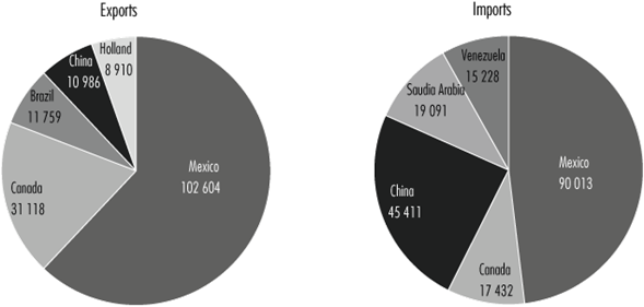
Note: * US$ million.
Source: US Department of Commerce.
Figure 1 Countries of destination of gross TX* exports and imports
The state of TX has the longest stretch of international border between the US and Mexico and the largest number of active land ports of entry, making it the first trading partner of MX and vice versa. Figure 1 presents the gross value data of TX exports and imports by country (top five countries) in 2013.
As shown in the figure above, TX's gross exports to MX amounted to US$102,634 million in 2013; in other words, TX directed 36% of its total exports to MX. At the same time, TX imports an amount of US$90,013 million from MX, in other words, a share of almost 30% of its gross state imports.
Figure 2 shows the foreign trade between TX and MX, breaking down final goods according to the main economic sectors (the five main products) in 2013.
Figure 2 shows the most relevant sectoral exports from TX to MX: mineral fuels (petroleum), oils and waxes, computer and electronic equipment, basic chemicals, machinery (excluding electrical), and other economic sectors. Meanwhile, the following stand out in decreasing order of importance in the sectoral imports of TX from MX: mineral fuels (petroleum), oils and waxes; computers and electronic equipment; transportation equipment and parts; machinery, chemical products; and other economic sectors.
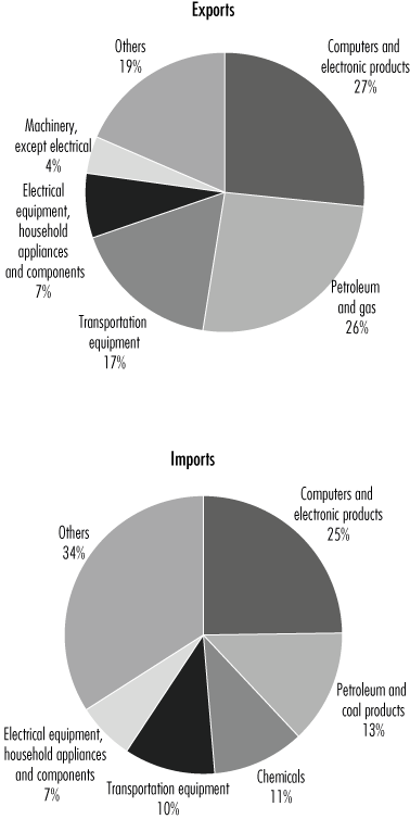
Note: * US$ million.
Source: US Department of Commerce.
Figure 2 Distribution by export and import products from TX to MX*
Regarding the state of CA, it has the smallest stretch of international border between the two countries; it is the second largest trading partner of MX and vice versa. Figure 3 shows the gross value of CA exports and imports by country (top five countries) in 2013.

Note: * US$ million.
Source: US Department of Commerce.
Figure 3 Countries of destination of CA's gross exports and imports*
As shown in figure 3, MX is the primary export market for CA. CA exports to MX totaled US$24,378 million in 2013, representing 14.2% of the total. Meanwhile, CA imports from MX amounted to US$36,128 million, representing 9.5% of total state imports for that year.
Figure 4 shows the foreign trade of CA and MX broken down by final goods according to the main economic sectors (the five main products).
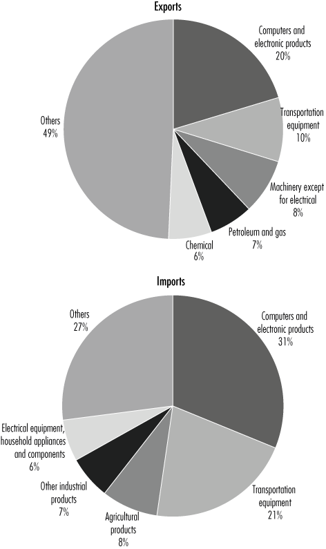
Note: * US$ million.
Source: US Department of Commerce.
Figure 4 Distribution by product of CA exports and imports*
The last two figures show that the five main exports from CA to MX were computer and electronic equipment, transportation vehicles, machinery (excluding electrical), automatic voice and image or data machines, and manufactured food products. Meanwhile, the five main imports of CA from MX for the same year were transportation vehicles, mineral fuels (petroleum), oils and waxes, automatic data processing machines, and automatic voice and image machines.
Based on the above, in 2013, TX-MX bilateral gross trade amounted to nearly US$192,907 dollars. While for CA-MX, reciprocal trade was US$60,605 million and CA's trade deficit with MX was US$11,649 million. In addition, TX-MX has an energy-technology trade pattern, while CA-MX has a technology-energy trade pattern.
Nevertheless, it can be noted that most of the trade between TX- MX and CA-MX is bidirectional within basically the same class of goods, suggesting an extensive production-sharing process that generates a series of global value chains, resulting in components manufactured in TX and CA being assembled or processed in MX and shipped back to TX and CA and vice versa.
In summary, the value and composition of the gross flow of imports and exports, as well as the gross trade balance, which are conventional measures of foreign trade based on the registration of goods produced entirely by a single country, are unreliable for analyzing the productive and commercial reality related to the current scheme based on the supply of intermediate goods, which are incorporated in the shared production processes between TX, CA, and MX.
3. GLOBAL INTERREGIONAL INPUT-OUTPUT MODEL AND STATISTICAL SOURCES
The global interregional input-output model represents the sectoral production system of two or more countries that explains the levels of intermediate and final exports based on the demand for intermediate and final imports of these countries and the rest of the world. Such models can be the result of a combination of two or more national economies to form a larger (supranational or global) economic unit, or they can be the result of an aggregate regional subdivision into groups of two or more economic entities, which do not necessarily coincide with a political unit. In the latter sense, the economies of TX-MX and CA-MX can be aggregated to form uniform regions (country-states) from a structural point of view.
By constructing the global interregional input-output matrices for TX-MX and CA-MX, it was deemed desirable that the level of sectoral aggregation be as detailed as possible. For the states of TX and CA, the matrices estimated by IMPLAN (Minnesota Implan Group [MIG], 2017) for 2013 were used, with a sectoral structure of 526 sectors. In the case of MX, the official Mexican input-output matrix for 2012 (INEGI, 2014), broken down to the four-digit level of the North American Industrial Classification System (SCIAN), composed of 261 sectors, was used.
It is worth mentioning that the Mexican matrix was updated to 2013 to match the US state matrices and to temporally coincide with the year to which the 2014 economic center data refers. The Mexican matrix was updated using the RAS technique,2 which consists of applying a bi-proportional iterative process based on the official base matrix and the availability of the values of the aggregates by row and column for the "desired" year in order to match the sum of the values of the sectoral interactions contained in the Mexican matrix with the aggregates of the borders of the Mexican matrix for the year to be estimated (Lahr and De Mesnard, 2004; INEGI, 2014). The data for the border aggregates of the official matrix for 2013 were taken from the 2014 economic census statistics (INEGI, 2014).
For the homologation of the TX-MX and CA-MX integrated interregional intersectoral matrices, sectoral compatibility of the individual matrices was sought. Of the 526 sectors, 488 fully matched at the four-digit level of the SCIAN,3 and the remaining 38 combined activities from several sectors were assigned using a weighting based on their relative participation in the aggregate using economic census data. This process resulted in 259 sectors. Consequently, the compatibility of activities between the two models required minor adjustments in the classifications, resulting in 247 economic sectors of activity.
The matrices were also reconfigured to a classification compatible with foreign trade. For this purpose, constructing the matrices required the estimation of trade flows between both US and Mexican state entities at the interaction level of individual sectors. The reasoning behind the estimation of the foreign trade matrices begins by considering that trade between TX-MX and CA-MX is already part of the import and export aggregates of the matrices of each political unit. Therefore, its incorporation into the matrix initially considers subtracting trade flow values from the import and export totals of the TX-MX and CA-MX matrices as appropriate.
Below, the overall TX-MX and CA-MX interregional matrices are presented in aggregate form in Tables 1 and 2, respectively. This representation of the basic structure of the global interregional intersectoral matrix allows us to quantify by origin and destination the linkages observed between the productive (intermediate and final) and commercial (internal and external) activities of both economies of TX-MX or CA-MX and the global economy.
Tables 1 and 2 show the global value chains contained in the bilateral-sectoral trade flows in order of importance of the values that appear in each quadrant of the global interregional matrix. These matrices make it possible to reconstruct the complete path of production and trade, from its initial stages to its final destination, breaking down the contribution of value at each stage.
Table 1 Aggregate representation of the TX-MX global interregional matrix, 2013 (US$ millions)
| Intermediate demand | Final demand | Total availability | |||||
| Texas | México | Texas | México | Exports to the rest of the world | Exports to the rest of the country | ||
| Texas | 919 908 | 69 644 | 969 208 | 20 679 | 114 811 | 694 845 | 2 796 093 |
| México | 64 461 | 633 529 | 37 552 | 1 145 837 | 286 107 | 2 166 486 | |
| Imports from the rest of the world | 404 580 | 232 615 | 289 635 | 83 724 | |||
| Value added | 1 408 144 | 1 225 461 | 138 959 | ||||
| Total production | 2 796 093 | 2 166 486 | 5 101 538 | ||||
Source: Compiled by the authors
Table 2 Aggregate representation of the CA-MX global interrgional matrix, 2013 (US$ millions)
| Intermediate demand | Final demand | Total availability | |||||
| California | México | California | México | Exports to the rest of the world | Exports to the rest of the country | ||
| California | 1 087 655 | 24 989 | 1 439 568 | 11 140 | 180 282 | 700 800 | 3 444 435 |
| México | 6 192 | 633 529 | 18 187 | 1 145 837 | 360 505 | 2 164 249 | |
| Imports from the rest of the world | 404 367 | 280 270 | 336 184 | 97 262 | |||
| Value added | 1 946 221 | 1 225 461 | 250 010 | ||||
| Total production | 3 444 435 | 2 164 249 | 5 858 693 | ||||
Source: Compiled by the authors.
4. GLOBAL VALUE CHAIN ACCOUNTING METHODOLOGY
All analysts now point out that competition is based on the value added that countries can place in foreign markets, which export not only final goods but also intermediate goods. This implies that the rise of global value chains is one of the major transformations in the global economy (Hopkins and Wallerstein, 1977; Gereffi, 1989). Many analysts use the global interregional input-output model to compute the value added of gross exports (Koopman et al., 2012 and 2014; De la Cruz et al., 2010; Johnson and Noguera, 2012a; Steher, 2013; OECD, 2013; Borin and Mancini, 2015; Banxico, 2016; Wang et al., 2014; Solaz, 2016, and others).
In this analytical framework and considering the dynamics of sectoral articulation given by the bilateral relationship between MX and the US, we find the paper by Murillo-Villanueva et al. (2022), who present evidence that the Mexican economy, mainly in the manufacturing area, has the lowest composition of domestic value added in its export sectors of the entire North American bloc. In the same vein and adding regulatory effects of sectoral articulation derived from economic integration in the North American bloc, we find the work of Fujii and Cervantes (2013 and 2017) and Gaytán-Alfaro (2022). They reiterate the empirical evidence of the scarce integrating and multiplier effect (measured by value aggregation nodes) that the performance of the Mexican export apparatus has had on the domestic market.
Koopman et al. (2012 and 2014) pioneered the use of the global intersectoral interregional model (using the WIOD database (Timmer et al., 2015 and 2016)) to decompose a country's gross exports into embedded value-added chains and those values counted twice using a unified framework. Conceptually, the components can be grouped into four basic categories: 1) direct domestic value added contained in gross exports, similar to "value-added exports" as defined by Johnson and Noguera (2012b); 2) domestic value added that is initially exported, but eventually returns home. While these exports are not part of a country's "value added", it is part of the exporting country's GDP; 3) direct foreign value added that is used in the production of a country's exports and is eventually absorbed by other countries; and 4) what the authors call "pure double-counted terms" derived from trade in intermediate goods that cross international borders several times. These basic components or categories of the global value-added chain contained in gross exports are shown in Figure 5.

Source: Koopman et al. (2014) and Wang et al. (2014, p. 23; 2018).
Figure 5 Breakdown of Gross Exports: Basic Categories
Subsequently, Wang et al. (2014 and 2018) made another methodological contribution related to the possibility of breaking down the bilateral gross trade balance at the sectoral level according to the origin or destination of the incorporated value added. Based on a global interregional intersectoral matrix for N countries and n sectors, they propose breaking down the value added of gross exports into different demands (intermediate or final) and trade routes (local or foreign). Moreover, to further refine the breakdown, they make an important distinction between backward and forward industrial linkages, which makes it possible to break down total intermediate trade flows according to their final absorption destination at the bilateral sector level. As a result, the separation of value added by backward versus forward industrial linkages is a conceptual advance that allows us to trace the structure of international shared production bilaterally at the disaggregated level.
The breakdown of the 16 value-added flows proposed by the authors is a long and tedious algebraic process. Due to space constraints, we cannot present the full derivation (the breakdown equation of the gross exports value added is presented by Wang et al. (2014)). We offer the 16 terms of the breakdown of value added of exports directed from TX or CA (TX/CA) to MX and give a simple interpretation of each component.
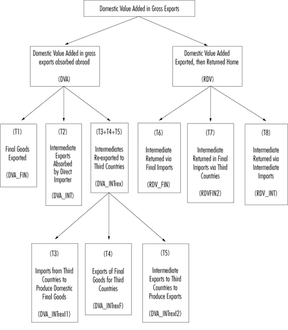
Figure 6 shows the first eight terms that refer to components of domestic value added encompassed in gross exports from TX/CA and MX. Component T1 (labeled as DVA_FIN) refers to the direct domestic value added contained in gross exports of final goods from TX/CA to MX. The T2 component (labeled as DVA_INT) shows the domestic value added used in gross exports by TX/CA to produce final goods ultimately consumed in TX/CA. The T3+T4+T5 component (labeled as DVA-INTex) is composed of three categories: a) component T3, which is the domestic value added of intermediate exports that are re-exported to a third location for the production of final goods (labeled as DVA_INTrex(1); b) component T4 which is the domestic value added implicit in intermediate exports used by TX/CA for final exports to third locations (labeled as DVA_ INTrexF); and, c) component T5 which is the domestic value added embedded in TX/CA's intermediate exports to produce intermediate goods exported to third places (labeled as DVA_INTrex(2)). Component T6 (labeled RDV_FIN) comprises the domestic value added that returns to TX/CA in the form of final goods from MX (labeled RVA_FIN). Component T7 contains the domestic value added that returns to MX in the form of imports of final goods from third places (labeled as RVA_FIN2) and, finally, component T8 is the domestic value added that returns to MX through intermediate imports to produce local goods (labeled as RVA_INT).
Figure 7 shows the terms that comprise the remaining eight terms of the external value added embodied in the gross exports of TX/CA and MX.
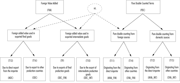
Figure 7 above establishes that component T9 (labeled as DDA_FIN) is a double-counting term generated by producing final goods exports. Component T10 (labeled as DDA_INT) is a pure double-counting term caused by exports of intermediate inputs. Component T11 (labeled as MVA_FIN) is the foreign value added imported from MX and included in the final exports from TX/CA to MX. The T12 component (labeled as OVA_FIN) is the foreign value added imported from a third place contained in intermediate exports from TX/CA to MX. The T13 component (labeled MDC) results from double counting the direct importer's value added for exports from the country of origin. The T14 term (labeled as OVA_FIN) is foreign value added imported from a third place contained in final exports from TX/CA to MX. The T15 term (labeled as (OVA_INT) is third country value added in intermediate exports; and finally, the T16 term (labeled as ODC) is a double count of third place value added in TX/CA exports.
At this point, we need to highlight some specific features of the methodology of the commercial value added breakdown developed by Wang et al. (2014 and 2018) and highlighted by Lopez (2019). Finally, it permits the calculation of a country's trade balance in terms of traded value added and not gross exports. Likewise, the algebraic breakdown permits the identification of the influence on the final demand of third countries in bilateral trade balance (De Gortari, 2017). Furthermore, it captures the breakdown not only at the bilateral level but also at the sectoral level. However, it does not permit the quantification of the value-added content of gross exports measured by the ratio between domestic value-added exports and gross exports (Johnson and Nogueira, 2012a), given that its direct calculation results in inconsistencies at the bilateral-sectoral level.
Likewise, several general characteristics of using the global interregional input-output model as a tool to analyze the multilateral interrelations of foreign trade should be highlighted (López, 2019). The first characteristic concerns the proportionality assumption used to distribute inputs to produce the different economic branches of activity (De Gortari, 2017; Puzzello, 2012). The second characteristic is related to the process of constructing the intersectoral and interregional matrices since transformations need to be made to the original technical coefficients, either to update and/or balance them to achieve global consistency. It is also related to the process of harmonizing the systems of national accounts across countries (Dietzenbacher et al., 2013). The third characteristic is that the production functions are degree one homogeneous and do not allow for external factors. In other words, constant returns to scale are assumed and external economies and diseconomies are explicitly excluded (Miller and Blair, 2009).4
In summary, we present the concepts developed by Wang et al. (2018) to separate the flows of value added embodied in bilateral-sectoral trade between TX-MX and CA-MX and highlight some advantages/disadvantages of using the methodology.
5. RESULTS
To estimate and analyze the particularities of the productive and commercial linkage of the TX-MX and CA-MX economies for 2013 from the perspective of the embodied flows of value added at the bilateral-sectoral level, it can be established as a first analysis of the breakdown of value added in the basic categories.
Tables 3 and 4 show the results of the condensed breakdown of the value added embodied in bilateral trade between TX-MX and CA-MX in 2013.
From the information recorded in Table 3, firstly, it can be seen that the direct value added contained in gross exports from TX to MX amounts to US$57,421 million, and in gross exports from MX to TX is equal to US$63,235 million. This, of course, does not consider whether the trade of goods is for intermediate or final use nor whether the destination is local or foreign. Second, the return value added from TX to MX is worth US$3,752 million, while from MX to TX, it is US$2,098 million. Third, the direct foreign value added used in exports from TX to MX is equivalent to US$45 214 million and the direct foreign content of exports from MX to TX is US$26 891 million; of course, noting that TX buys a significant portion in the rest of the US. In fourth place is the double counting derived from the trade of intermediate goods that cross international borders several times from TX to MX and vice versa, amounting to US$2,350 million.
Table 3 Breakdown of value added in basic categories, TX-MX, 2013 (US$ millions)
| Components | Bilateral trade | |||
| TX-MX | MX-TX | |||
| DVA | Domestic Value Added | 57 420.9 | 63 235.0 | |
| RVA | Return Value Added | 3 752.1 | 2 097.8 | |
| FVA | Foreign Value Added | 45 213.8 | 26 891.1 | |
| PDC | Pure Double Counting | 2 350.1 | 2 350.1 | |
| Gros Exports | 102 634.7 | 90 126.1 | ||
Source: Compiled bu the authors.
The information in Table 4 shows, first, that the direct value added included in gross exports from CA to MX amounts to US$13,451 million and from MX to CA US$21,484 million, without distinguishing whether they are raw materials or final goods, whether local or foreign. Second, domestic value added, initially exported from CA to MX but eventually returns home, is $2,098 million and from MX to CA, $1,333 million. Third, the direct foreign value added that is used in the production of exports, and which is finally absorbed by other countries or regions of the US economy from CA or MX is $10,493 million, and from MX to CA $14,565 million, noting that CA buys a significant amount in the rest of the US. In fourth place, there is the double counting derived from the trade of intermediate goods that cross international borders several times from CA to MX or from MX to CA, totaling US$2,350 million between both geographical areas.
Table 4 Breakdown of value added in basic categories, TX-MX, 2013 (US$ millions)
| Components | Bilateral Trade | ||
| CA-MX | MX-CA | ||
| DVA | Domestic Value Added | 13 451.3 | 21 483.9 |
| RVA | Return Value Added | 0.0 | 0.0 |
| FVA | Foreign Value Added | 10 493.3 | 14 564.7 |
| PDC | Pure Double Counting | 124.5 | 124.5 |
| Gross Exports | 23 944.5 | 36 048.6 | |
Source: Compiled by the authors
Based on the above, it can be deduced that a high content of MX's gross exports come from TX, CA, or from outside these US states. The separation and analysis of two-way international trade flows between TX-MX and CA-MX need to be expanded, including whether the value added comes from intermediate or final goods and whether it is internal or external. Tables 5 and 6 show the results of the expanded category breakdown of the value added contained in bilateral trade between TX-MX and CA-MX in 2013. The results were achieved by applying the "decompr" library (Quast and Kummritz, 2015) implemented in the R software (R Core Team, 2018).
The first five items in table 5 refer to components of the value added encompassed in the gross exports of final goods from TX to MX. T1 (DVA_FIN) indicates that US$14,099 million corresponds to the direct Texan value added contained in final goods exports shipped from TX to MX. T2 (DVA_INT) indicates that US$26,676 million corresponds to the Texan value added used in intermediate exports by TX to produce final goods ultimately consumed in MX. The sum of the terms T3 (DVA_INTex) + T4 (DVA_INTrex(1) + T5 (DVA-INTrexF) shows that $14,458 million is the share of Texan value added that comes from elsewhere, both from the rest of the US and from abroad.5 T6 (RVA_FIN) reveals that $1,573 million comprises the Texan value added that returns to TX as final goods from MX. T7 (RVA_FIN2) equals zero in imports of final goods from third countries, and T8 (RVA_INT) shows that US$595 million is the Texan value added, returning to MX as intermediate imports to produce Mexican goods.6
Table 5 Breakdown of value added in basic categories, CA-MEX, 2013 (US$ millions)
| Components | Acronyms | Bilateral trade in 2023 | |
| TX-MX | MX-TX | ||
| T1 | DVA_FIN | 14 098.7 | 17 432.4 |
| T2 | DVA_INT | 26 676.4 | 11 123.2 |
| T3 | DVA_INTrexI1 | - | - |
| T4 | DVA_INTrexF | 14 547.9 | 30 927.2 |
| T5 | DVA_INTrex12 | - | - |
| T8 | RDV_INT | 594.8 | 3 033.8 |
| T6 | RDV_FIN | 1 503.0 | 718.3 |
| T7 | RDV_FIN2 | - | - |
| T14* | OVA_FIN | - | - |
| T11 | MVA_FIN | 718.3 | 1 503.0 |
| T15* | OVA_INT | - | - |
| T12 | MVAINT | 3 033.8 | 594.8 |
| T9 | DDCFIN | 958.5 | 1 118.7 |
| T10 | DDCINT | 125.6 | 147.3 |
| T16* | ODC | - | - |
| T13 | MDC | 1 266.0 | 1 084.1 |
| T14+T15+T16 | Resto del mundo | 39 111.6 | 22 443.2 |
| Total exports | 102 634.7 | 90 126.1 | |
Note: * acronyms explained in the methodology and related in figure 6 and 7.
Source: Compiled by the authors
T9 (DDC_FIN) and T10 (DDC_INT) indicate that US$959 million and 126 million are due to pure double counting caused by TX exports of final goods and intermediate inputs, respectively. T13 (MVA_INT) states that $1,266 million is the foreign value added imported from a third location contained in TX intermediate exports to MX.7 T11 (MVA_FIN) and T12 (MVA-INT) note that $718 million and $3,034 million are the double counting of TX value added from final goods and intermediate inputs. Finally, T14 (OVA_FIN) + T15 (OVA_INT) + T16 (ODC) add up to US$39,112 million, corresponding to foreign value added in TX final and intermediate third country exports.
Table 6 highlights the value-added components of CA-MX bidirectional trade. It shows that $9,922 million corresponds to direct Californian value added contained in exports of final goods shipped from CA to MX, and another $6,692 million corresponds to Californian value added used in exports of intermediate goods by CA to produce final goods and ultimately to be consumed in CA. In addition, $1,433 million is the portion of Californian value added from elsewhere: the rest of the US and abroad. The other components of CA exports to MX are US$364 million, corresponding to the Californian value added that returns to CA in the form of final goods from MX and US$70 million is the Californian value added that returns to MX through intermediate imports to produce Mexican goods. Around US$1 million and US$77 million are due to pure double counting caused by final and intermediate input exports, respectively. US$41 million is the foreign value added imported from a third location in intermediate exports from CA to MX. Finally, T14 (OVA_FIN) + T15 (OVA_INT) + T16 (ODC) total US$10,369 million, corresponding to foreign value added in final and intermediate Texan exports from third places.
Table 6 Breakdown of value added in broad categories, CA-MEX, 2013 (US$ millions)
| Components | Acronyms | Bilateral trade in 2013 | |
| CA-MX | MX-CA | ||
| T1 | DVA_FIN | 9 922.3 | 7 090.2 |
| T2 | DVA_INT | 6 692.2 | 2 014.7 |
| T3 | DVA_INTrexI1 | - | - |
| T4 | DVA_INTrexF | 1 433.5 | 7 267.7 |
| T5 | DVA_INTrex12 | - | - |
| T8 | RDV_INT | 29.6 | 70.2 |
| T6 | RDV_FIN | 51.1 | 363.6 |
| T7 | RDV_FIN2 | - | - |
| T14* | OVA_FIN | - | - |
| T11 | MVA_FIN | 363.3 | 51.1 |
| T15* | OVA_INT | - | - |
| T12 | MVAINT | 70.2 | 29.6 |
| T9 | DDCFIN | 40.5 | 77.1 |
| T10 | DDCINT | 0.8 | 6.1 |
| T16* | ODC | - | - |
| T13 | MDC | 83.2 | 41.3 |
| T14+T15+T16 | Resto del mundo | 10 368.8 | 14 440.2 |
| Total exports | 24 378.3 | 36 129.4 | |
Note: * acronyms explained in the methodology and related in figure 6 and 7.
Source: Compiled by the authors.
Meanwhile, the criterion for separating bi-directional international trade flows between TX-MX and CA-MX was extended to include the origin or destination of value added in trade between these locations.
The tables suggest that MX presents a concentrated pattern in the use of foreign intermediate goods; in other words, it has a high degree of dependence on intermediate goods from TX, CA, and foreign countries. Meanwhile, TX and CA are positioned as suppliers of intermediate goods for exports and MX in final goods. Consequently, an increase in TX and CA production and trade in MX has a low impact (low export multiplier effects) in MX.
Finally, the value added chain breakdown was estimated and analyzed by incorporating backward versus forward sectoral linkages. This conceptual advance allows us to trace the pattern of international sectoral production sharing at the bilateral level between TX-MX and CA-MX. Tables 7 and 8 present the breakdown of the gross trade balance into sectors of activity (we show the 15 most important sectors). From the information contained therein, we can confirm the existence of a similar dynamic at the sectoral level as at the aggregate level. In other words, the aggregate trade surplus of TX with MX leads to a sectoral trade surplus between these geographical areas.
The information in Table 7 shows that TX-MX bilateral productive integration is concentrated in a few sectors of activity through the trade exchange to which their key intermediate goods give rise. For example, mineral fuels (petroleum), oils and waxes, basic chemical products, electronic components, electrical equipment and parts, computer equipment and parts, machinery except for electrical, aerospace equipment, automotive vehicles; and meat products. All these broadly defined sectors show a high utilization of Texan inputs (directly (DVA_INT) and indirectly (DVA_INTrex)) amounting to 50% of the total required production inputs. These are the most vertically integrated sectors in terms of the value of the trade balance (gross bilateral trade).
Tabla 7 Resultados del desglose de valor agregado en el comercio TX-MX por principales sectores (US$ millones)
| Code | Description | Domestic Contentent | Foreign Content | Gross Bilateral Trade | |||||||||
| Domestic Value Added (DVA) | Double count | Foreign Value Added (FVA) | Double Count | Rest of the World | |||||||||
| Value Added in Exports | DVA reexported | DVA returned | |||||||||||
| DVA_FIN | DVA_INT | DVA_INT rep | RVD_FIN | RVD_INT | DDC | MVA_FIN | MVA_INT | MDC | |||||
| 3241 | Manufacture of petroleum and coal products | 330 | 9 617 | 1 889 | 120 | 86 | 193 | 71 | 2 053 | 487 | 5 833 | 20 679 | |
| 3251 | Manufacture of basic chemicals | 331 | 3 540 | 1 419 | 138 | 82 | 210 | 24 | 257 | 135 | 5 744 | 11 879 | |
| 3344 | Manufacture of electronic compoents | 82 | 1 257 | 5 040 | 371 | 105 | 156 | 3 | 51 | 231 | 1 247 | 8 545 | |
| 3331 | Manufacture of agricultural, construction and mining and quary machinery | 2 229 | 863 | 219 | 24 | 13 | 22 | 112 | 43 | 14 | 2 115 | 5 653 | |
| 3361 | Manufacture of automobiles and trucks | 1 743 | 17 | 17 | 6 | 0 | 1 | 319 | 3 | 4 | 2 437 | 4 548 | |
| 3252 | Manufacture of synthetic resins and rubbers, and chemical fibers | 2 | 876 | 800 | 78 | 36 | 31 | 0 | 42 | 46 | 1 694 | 3 606 | |
| 4811 | General-purpose motor transportation | 1 938 | 0 | 0 | 0 | 0 | 0 | 69 | 0 | 0 | 712 | 2 718 | |
| 3345 | Manufacture of measuring, control, navigation and medical electronic instruments and equipment | 753 | 349 | 563 | 69 | 26 | 21 | 23 | 11 | 21 | 780 | 2 616 | |
| 3339 | Manufacture of other machinery and equiment for general industry | 816 | 373 | 256 | 21 | 12 | 15 | 32 | 14 | 12 | 848 | 2 397 | |
| 3364 | Manufacture of aerospace equipment | 412 | 168 | 483 | 44 | 13 | 40 | 17 | 7 | 23 | 1 055 | 2 262 | |
| 3341 | Manufacture of computers and peripheral equipment | 664 | 120 | 392 | 31 | 11 | 18 | 40 | 7 | 27 | 841 | 2,149 | |
| 332 | Manufacture of other metal products | 3 | 589 | 582 | 49 | 29 | 35 | 0 | 26 | 31 | 481 | 1 825 | |
| 3342 | Manufacture of communication equipment | 430 | 140 | 495 | 48 | 10 | 17 | 14 | 5 | 19 | 470 | 1 649 | |
| 3363 | Manufacture of auto parts for motor vehicles | 13 | 410 | 331 | 83 | 11 | 16 | 1 | 27 | 29 | 684 | 1 603 | |
| 3116 | Slaughtering, packing and processing of meat, poultry, and other editable animals | 715 | 148 | 20 | 6 | 1 | 2 | 38 | 8 | 2 | 574 | 1 513 | |
Source: Direct information prepared based on Wang et al. (2018).
Such productive complementarity with MX occurs in the sector of mineral fuels (petroleum), oils and waxes with a high imported value of inputs from this country (MVA_INT). Next in order of importance are the sectors of basic chemical products, electrical equipment and parts, and computer equipment and parts defined in a broad sense, which enable an indirect link from these sectors.
The size of the productive asymmetry between TX-MX is reflected in the global value chains of the sectors of basic chemicals, electrical equipment and parts, and computer equipment and components with a significantly lower weighting in MX in terms of productive input requirements close to 25%. These results are due, on the one hand, to the low level of productive inputs imported by TX from MX. On the other hand, for the Mexican sectors, the aforementioned Texan sectors represent their leading suppliers.
The data included in Table 8 show the bilateral-sector integration of CA-MX. According to the volume of incorporated intermediate inputs, the production pattern is concentrated in electronic components, mineral fuels (petroleum), oils and waxes, automotive vehicles, basic chemicals, communication equipment, and medical equipment. As in the previous case, these more broadly defined sectors represent high direct (DVA_INT) and indirect (DVA_INTrex) Californian integration. The total required intermediate inputs amount to 69% of the total.
Table 8 Results of the breakdown of value added in CA-MX trade by main sectors (US$ millions)
| Code | Description | Domestic Content | Foreign Content | Gross Bilateral Trade | |||||||||
| Domestic Value Added (DVA) | Double count | Foreign Value Added (FVA) | Double count | Rest of the World | |||||||||
| Value added in exports | DVA Re-Exported | DVA returned | |||||||||||
| DVA_FIN | DVA_INT | DVA_INT rep | RVD_FIN | RVD_INT | DDC | MVA_FIN | MVA_INT | MDC | |||||
| 3344 | Manufcature of electronic components | 339 | 1 421 | 1 068 | 2 759 | 1 475 | 409 | 7 | 28 | 114 | 1 492 | 9 110 | |
| 3241 | Manufacture of petroleum and coal products | 0 | 4 392 | 351 | 272 | 363 | 96 | 0 | 300 | 75 | 3 191 | 9 037 | |
| 3363 | Manufacture of motor vehicle parts | 143 | 2 998 | 486 | 2 315 | 613 | 185 | 3 | 64 | 78 | 1 533 | 8 416 | |
| 3251 | Manufacture of basic chemical products | 126 | 2 513 | 226 | 276 | 530 | 131 | 3 | 52 | 24 | 951 | 4 833 | |
| 3252 | Manufacture of synthetic resins, rubbers, and chemical fibers | 0 | 1 261 | 210 | 492 | 546 | 125 | 0 | 26 | 28 | 742 | 3 430 | |
| 3361 | Manufacture of automobiles and trucks | 2 264 | 16 | 3 | 20 | 3 | 1 | 100 | 1 | 1 | 766 | 3 175 | |
| 3342 | Manufacture of communication equipment | 765 | 159 | 130 | 388 | 176 | 54 | 15 | 3 | 15 | 593 | 2 300 | |
| 3341 | Manufature of computers and peripheral equipment | 691 | 453 | 132 | 299 | 168 | 46 | 14 | 9 | 14 | 440 | 2 266 | |
| 3339 | Manufacture of other machinery and equipment for general industry | 949 | 397 | 55 | 91 | 123 | 34 | 19 | 8 | 6 | 351 | 2 031 | |
| 3345 | Manufacture of measuring, control, navigatio, and electronic medical equipment instruments | 445 | 178 | 67 | 178 | 122 | 35 | 7 | 3 | 6 | 201 | 1 242 | |
| 3336 | Manufacture of internal combustion engines, turbines and transmissions | 53 | 426 | 83 | 191 | 128 | 50 | 2 | 12 | 13 | 253 | 1 211 | |
| 3261 | Manufacture of plastic products | 121 | 402 | 69 | 174 | 124 | 32 | 2 | 6 | 6 | 183 | 1,117 | |
| 3353 | Manufacture of electric power generation and distribution equipment | 68 | 122 | 38 | 82 | 96 | 27 | 2 | 3 | 7 | 99 | 544 | |
| 3329 | Manufacture of other metal products | 15 | 187 | 33 | 85 | 93 | 26 | 0 | 3 | 4 | 78 | 524 | |
| 3359 | Manufacture of other electrical equipment and accessories | 47 | 114 | 38 | 98 | 82 | 24 | 1 | 3 | 7 | 104 | 518 | |
Source: Direct information prepared based on Wang et al. (2018)
According to the figures in the table above, it can be deduced that CA has higher export multiplier effects than MX, both direct and indirect because the latter uses a high amount of intermediate inputs in the productive process. The case of the previous sectors is where a higher content of Californian inputs is observed.
6. CONCLUSIONS
The US and Mexican economies are closely linked not only because of the high degree of interaction between the US economy and the Mexican economy but also because they jointly produce for the world market.
In 2013, TX and CA were MX's main trading partners. The bilateral-sectoral trade balance shows that TX and CA specialize in intermediate goods exports and MX in final goods; impacting the latter with low export multipliers. MX has a high degree of dependence on intermediate goods from TX, CA and third places, implying lower foreign exchange earnings per dollar exported. Both TX-MX and CA-MX have a diversified trade pattern (albeit in different proportions). While TX-MX trade has historically been in energy with technology gaining ground, CA-MX trade has traditionally been in goods with technological content, with energy goods currently gaining ground. For this reason, we also analyzed the value-added chain breakdown calculations incorporating backward versus forward sectoral linkages. This conceptual advance allows us to track the structure of international sectoral production sharing at the bilateral level between TX-MX and CA-MX. In particular, based on this analysis, the evidence of low multiplier effects in the domestic market of Mexican exports to TX and CA derives from the fact that the value chains that sustain them are configured by intermediate supply structures that support economic circuits geographically located in said states of the American Union and the energy and technological fields, respectively. This means eroding the dragging and driving effects of the domestic economic activity that potentially resides in the dynamism of the Mexican export apparatus. This scenario is expressed in the configuration of productive nodes with greater value aggregation dynamics in TX and CA, as well as in the deterioration of the capacity to translate the expansion of gross value added in Mexico (highly determined by exports) into greater remuneration to the factors of production.
REFERENCES
Arreola, J. (2015). California y Texas: dos fronteras de progreso. World Economic Forum, 2015. https://es.weforum.org/agenda/2015/06/californiay-texas-dos-fronteras-de-progreso/ [ Links ]
Borin, A. y Mancini, M. (2015). Follow the valued added; Bilateral gross exports accounting. Working Paper, 1026, Bank of Italy. [ Links ]
Banxico (noviembre de 2016). Análisis del balance comercial manufacturero de Estados Unidos con México en términos de valor agregado. Extracto del Informe Trimestral julio-septiembre. [ Links ]
De Gortari, A. (2017). Disentangling global value chains. Meeting Papers 139 Minneapolis Society for Ecomomic Dynamics. [ Links ]
De la Cruz, J., Koopman, R., Wang, Z. y Wei, S. (2010). Estimating foreign value-added in Mexico’s manufacturing exports. US International Trade Commission, Office of Economics. Working Paper (2011-04A). https://www.usitc.gov/publications/332/EC201104A.pdf [ Links ]
De Mesnard, L. (1989). Note about the theoretical foundations of biproportional methods. Ninth International Conference on Input-Output Techniques, Keszthely. [ Links ]
Dietzenbacher, E., Los, B., Stehrer, R., Timmer, M. y de Vries, G. (2013). The construction of world Input-Output tables in the WIOD Project. Economic Systems Research, 25(1). https://www.tandfonline.com/doi/abs/10.1080/0 9535314.2012.761180 [ Links ]
Fuentes, N. A., Brugués, A. y González-König, G. (2020). Valor agregado en el valor bruto de las exportaciones: una mejor métrica para comprender los flujos comerciales entre Estados Unidos y México. Frontera Norte, 32(7). http://dx.doi.org/10.33679/rfn.v1i1.1990. [ Links ]
Fujii, G. y Cervantes M., R. (2013). México: valor agregado en las exportaciones manufactureras. Revista CEPAL, 109. https://repositorio.cepal.org/page/countries-regions [ Links ]
______ y Cervantes, M. (2017). The weak linkages between processing exports and the internal economy. The Mexican case. Economic Systems Research, 29(4).http://www.paginaspersonales.unam.mx/files/249/Publica_20180216162955.pdf [ Links ]
Gereffi, G. (1999). International trade and upgrading in the apparel commodity chain. Journal of International Economics, 48(1).http://openscienceasap.org/wpcontent/uploads/2013/10/Gereffi_1999_Commoditychains1.pdf . [ Links ]
Gaytán-Alfaro, E. D. (2022). Integración económica de México al mercado común de América del Norte: un análisis insumo-producto multipaís en el marco normativo del T-MEC. Revista de Economía Mundial, (61 ).http://uhu.es/publicaciones/ojs/index.php/REM/article/view/5346 [ Links ]
Hopkins, T. y Wallerstein, I. (1977). Patterns of development of modern world systems. Review, I(2).https://www.jstor.org/stable/26918185 [ Links ]
Instituto Nacional de Estadística Geografía e Informática (INEGI) (2014). Sistema de Cuentas Nacionales de México. Desarrollo de la matriz de insumo producto 2012. http://www.inegi.org.mx/est/contenidos/proyectos/cn/mi p12/doc/SCNM_Metodologia_28.pdf [ Links ]
Johnson, R. C. y Noguera, G. (2012a). Accounting for intermediates: Production sharing and trade in value added. Journal of International Economics , 86(2). https://ideas.repec.org/a/eee/inecon/v86y2012i2p224236.html [ Links ]
______ y Noguera, G. (2012b). Proximity and production fragmentation. American Economic Review, 201(3).https://www.aeaweb.org/articl es?id=10.1257/aer.102.3.407 [ Links ]
Koopman, R., Wang, Z. y Wei, S. J. (2012). Tracing value-added and double counting in gross exports. Working Paper 18579. http://www.nber.org/ papers/w18579. [ Links ]
______, Wang, Z. y Wei, S. J. (2014). Tracing value-added and double counting in gross exports. American Economic Review, 104(2).https://www. aeaweb.org/articles?id=10.1257/aer.104.2.459 [ Links ]
Lahr, M. y De Mesnard, L. (June 2004). Biproportional techniques in InputOutput analysis: Table updating and structural analysis. Economic Systems Research , 16(2).https://www.researchgate.net/publication/227611840_Bi proportional_Techniques_in_Input-Output_Analysis_Table_Updating_ and_Structural_Analysis [ Links ]
López, R. (2019). Impacto de la demanda interna de terceros países en la balanza comercial de las manufacturas guatemalteca: El caso de las relaciones comerciales con Estados Unidos, México y El Salvador. Banca Central , ( 78). http://www.banguat.gob.gt/sites/default/files/banguat/Publica/Banca/BancaCentral78.pdf [ Links ]
Miller, R. E. y Blair, P. D. (2009). Input-Output analysis: Foundations and extensions (second ed.). Cambridge University Press. [ Links ]
Minnesota Implan Group (MIG) (2017). United States 2013 implant data. Minnesota Implan Group. [ Links ]
Murillo-Villanueva, B., Carbajal Suárez, Y. y Almonte, L. (2022). Valor agregado en las exportaciones manufactureras del TLCAN, 2005, 2010 y 2015. Un análisis por subsector. Análisis Económico, 37(95). https://www.redalyc.org/articulo.oa?id=41372042005 [ Links ]
Nagengast, A. J. y Stehrer, R. (2016). The great collapse in value added trade. Review of International Economics, 24(2). http://doi.org/10.1111/roie.12218 [ Links ]
OECD (2013). Towards green growth: monitoring progress-OECD Indicators. OECD. [ Links ]
Puzzello, L. (2012). A proportionality assumption and measurement biases in the factor content of trade. Journal of International Economics , 87(1). https://econpapers.repec.org/article/eeeinecon/v_3a87_3ay_3a2012 _3ai_3a1_3ap_3a105-111.htm [ Links ]
R Core Team (2018). R: A language and environment for statistical computing. R Foundation for Statistical Computing. Vienna, Austria. https://www.Rproject.org [ Links ]
Solaz, M. (2016). Cadenas globales de valor y generación de valor añadido: el caso de la economía española. Working Papers. Serie EC 2016-01, Instituto Valenciano de Investigaciones Económicas, S.A. (IVIE), 1. [ Links ]
Stehrer, R. (2013). Accounting relations in bilateral value added trade. Wiener Institute für Internationale Wirtschaftsvergleiche. [ Links ]
SMU Mission Foods (2019). Value added: A better metric to understanding TXMX trade flows. Proyecto Colaborativo entre UCSD, SMU y COLEF. Tijuana, B.C. México. [ Links ]
Timmer, M. P., Dietzenbeacher, E., Los, B., Stehrer, R. y de Vires, G. (2015). An illustrated user guide of the world Input-Output Database: The case of global automotive production. Review in International Economics, 23(3).https://www.ecb.europa.eu/home/pdf/research/compnet/CompNet_ ECB_WS3_Stehrer.pdf?955fe4ed6125589b82c9fe2bb997e619 [ Links ]
______, Los, B., Stehrer, R. y de Vires, G. (2016). An anatomy of the global trade slowdown based on the WIOD 2016 Release. GGDC Research Memorandum 162. University of Groningen. [ Links ]
Wang, Z. , Wei, S. y Zhu, K. (2014). Quantifying international production sharing at the bilateral and sector levels. Working Paper 19677. https://www.nber.org/system/files/working_papers/w19677/w19677.pdf [ Links ]
______, Wei, S. y Zhu, K. (2018). Quantifying international production sharing at the bilateral and sector levels, NBER Working Paper 19677. Cambridge National Bureau of Economics Research. [ Links ]
1This paper is a result of the Value Added: A Better Metric to Understanding TX-MX Trade Flows project funded by SMU Mission Foods TX-MX in 2019. Errors and omissions are the responsibility of the authors.
2 This method is a translation of the theory of matrix adjustment with restrictions to the estimation of input-output matrices (row and column totals). This adaptation was first used as a technique for updating the intermediate transactions matrix (De Mesnard, 1989).
3Sector approvals are based on Clouse, Candi. IMPLAN Industries and NAICS Correspondences available at https://support.implan.com/hc/en-us/articles/115009674428-IMPLAN-Industries-NAICS-Correspondences.
4It is important to mention that the relevance of these limitations is lower in ex-post time-cutting studies (Nagengast and Stehrer, 2016; Lopez, 2019).
6 Note that the sum of the five terms amounts to US$57,421 million corresponding to the basic category of Texas value added.
7 Note that the sums of the three terms add up to a total of US$3,752 million equal to the basic category of Texas return value added.
Received: October 21, 2022; Accepted: April 28, 2023
 Este es un artículo publicado en acceso abierto bajo una licencia Creative Commons
