


Servicios Personalizados
Revista
Articulo
 texto en
  Inglés (pdf)
 Artículo en XML
 Referencias del artículo
 Enviar artículo por email
Indicadores
-
 Citado por SciELO
 -
 Accesos
Links relacionados
-
 Similares en
SciELO
Similares en
SciELO
Compartir

 Permalink
Problemas del desarrollo
versión impresa ISSN 0301-7036
Prob. Des vol.53 no.209 Ciudad de México abr./jun. 2022 Epub 19-Sep-2022
https://doi.org/10.22201/iiec.20078951e.2022.209.69785
Articles
Capital flows and financial development: a view from developing countries
aNational Autonomous University of Mexico (UNAM), Faculty of Economics, Mexico. Email address: noemi.levy@gmail.com.
bNational Autonomous University of Mexico (UNAM), Faculty of Higher Learning-Acatlán, Mexico. Email address: alonsobt@yahoo.com.mx.
In Latin America, financial relations became more complicated and large companies were consolidated during the globalization phase. Interestingly, however, the capital market did not develop at the same pace, as the operations of large companies (multinationals and multilatinas) were not conducted via domestic financial institutions, but rather via bonds issued by international financial centers. In light of this, the article employs a panel data econometric model to measure the impact of capital flows (FDI and portfolio) on a set of financial and real sector indicators. Findings show that capital inflows did not contribute to financial development or economic growth.
Key Words: multinationals; financial markets; FDI; capital movements; panel data
En América Latina la complejización de las relaciones financieras y la consolidación de la gran empresa tuvo lugar durante el periodo de globalización, con la peculiaridad de que el mercado de capitales no se desarrolló a la par, ya que las operaciones de las grandes empresas (multinacionales y multilatinas) no se realizaron a través de las instituciones financieras domésticas, sino vía la emisión de bonos en los centros financieros internacionales. A partir de esta idea es que se realiza un modelo econométrico de datos de panel que mide el impacto de los flujos de capital (IED y cartera) en un conjunto de indicadores del sector financiero y real para mostrar que la entrada de capital no contribuyó al desarrollo financiero ni al crecimiento económico.
Palabras clave: multinacionales; mercados financieros; IED; movimientos de capital; datos de panel
Clasificación JEL: F23; E44; G15; CO1; C23
1. INTRODUCTION
The consolidation of large companies required developed financial markets which, by nature, promote speculative activities. It is assumed that the most relevant function of the financial structure in business development is the creation of credits. When these are channeled into the “real” sphere, they expand production and accumulation, though they can also be used to buy and sell financial securities in order to obtain financial gains. Non-bank financial institutions provide liquidity to illiquid assets and thus become a vehicle for distributing profits within the capitalist class (rentiers and investors).
Our take is that bank loans channeled to non-financial companies are linked to the expenditure of capital in circulation (Seccareccia, 2003) and the purchase of securities. Short-term non-monetary financial instruments (private and public bonds, both domestic or foreign) are kept to take on outstanding commitments as they have a resale value which does not substantially deviate from their par value. Meanwhile, long-term securities like stocks and long-term bonds (consols), generate liquidity and provide access to financial gains.
The analytical framework of this discussion is an oligopolistic structure in which large companies dominate and is inextricably linked to the capital market. The primary objective of this article is to analyze the relationship between financial development as expressed through financial complexity, large companies and the financial (in)stability of developing countries in Latin America.
The hypothesis to be tested is that the financial complexity in Latin America responded to the valuation needs of large foreign capital, thereby generating great instability. On the one hand, there was a large influx of foreign capital (Foreign Direct Investment-FDI and Foreign Portfolio Investment-FPI) with a reduced presence in domestic financial markets. Latin American non-financial corporations (multilatinas) also emerged in these markets with a reduced share. Big capital marginally operated in the region’s domestic bond and stock market and generated growing external debt with little economic growth.
Specifically, we argue the Latin American financial complexity responded to the movement of external capital caused by FPI in the first half of the 1990s and during the Global Financial Crisis of 2008 (GFC-2008). It sought to be valued in Latin America and was accompanied by FDI that installed itself in the most dynamic productive sectors. The peculiarity of this process is that the operations of large companies in the region failed in bringing about a strong expansion of its bond and stock market.
Then, in spite of this market’s development, its expansion into the international market, which deepened after the GFC-2008, did not achieve a high degree of complexity, resulting in growing external debt. Thus, the influx of foreign capital and dependence on external liquidity renewed developing countries’ dependence, as demonstrated by Luxembourg at the beginning of the 20th century (1913, chap. XXX).
This article is divided into five sections including the introduction. The second section presents a brief theoretical discussion on the development of large companies and their relationship with the financial market. In the third we review the development of the financial market in the region’s countries while paying close attention to the makeup of the market’s different segments in order to evaluate the depth and diversity of financial securities. The fourth section presents an econometric model that measures the impact of capital inflows (FDI and FPI) on a set of financial and real sector indicators. Finally, the fifth section presents our conclusions.
2. LARGE COMPANIES AND FINANCIAL MARKET DEVELOPMENT
LARGE COMPANIES
The main feature of large companies in the nineteenth century is the separation of ownership and corporate control. The sole owner and administrator of the company was replaced by a large number of bond and share-holders and a governing board which assumed control of the company and had the power to appoint a director. These conditions gave way to large corporations which distributed the property among a large number of people (shareholders) who were led by a governing board which exercised control. This nevertheless resulted in an aggregation and concentration of wealth. The strengthening of large enterprises is combined with the deepening of the financial market, which in turn increased production unit size and accelerated accumulation. Due to financial instability marked by periods of economic acceleration and great financial crises, the capital system’s oligopolistic phase was established at this time, replacing the economic stability of the 19th century known as the Gilded Age (Polanyi, 1944; Keynes, 1919).
Within this framework, profits were concentrated around the power group. This can accelerate, but also destabilize the financial system, even creating economic paralysis (the crises of 1929 and 2008). On the one hand this process guarantees large volumes of liquidity to companies. On the other hand, by issuing debt in order to access profits from variations in bond and share prices, it increases the debt of these entities and, if they default, can cause crises if their securities stop increasing in price, generating Minsky moments (1986).
This process is distinguished by the fact that the group that backs a corporation’s power makes decisions using other agents’ property without jeopardizing its own wealth. Thus, profits are not distributed proportionally among shareholders, according to the capital invested, but based on the power groups within the boards of directors. Obviously, this process is subject to strong contradictions as it dilutes ownership of the company, which in turn imposes a limit on the issuance of securities (Kalecki, 1971, chap. 9) and diversifies the forms of ownership (shares and property rights) through different types of shares: with and without voting rights, common and preferential, with and without par value. The process is also accompanied by certain policies regarding dividend distribution and the practices of buying back shares, all of which redistributes wealth in favor of the power groups.1
The rise of joint-stock companies reorganized the capitalist system, whose distinctive feature was a transition towards a concentrated oligopolistic phase. This diversified securities and deepened the financial system and deployed a wide variety of financial innovations, causing an increase in liquidity and a concentration of profits. In periods when financial capital dominates, mergers and acquisitions are strengthened, consolidating the large company which coexists with small and medium-sized companies (Steindl, 1945).
FINANCIAL STRUCTURE
The dominant paradigm places the stock market as a place for efficient intermediation. Here production relationships are ruled by scarcity of capital which is itself distributed among the most profitable projects via the mechanism of “correct” prices. So financial profits are possible given a set of productive factors where saving determines investment and those variables determine the natural interest rate and the productive factors’ mobility guarantees profit maximization. But this is as a consequence of ideal trades and “correct” prices generating a zero-sum game which financial bubbles and crises wipe out.
Modigliani and Miller (1958) point out that the financial structure does not modify corporations’ value in financial markets. Nevertheless, bank loans have advantages over non-bank financing due to tax considerations.
On the other hand, Fama (1991) assumed that capital market liquidity distribution favors certain players but only temporarily, asserting the random walk hypothesis. Meanwhile, Shiller (2000) questioned this assumption and proposed the existence of trends or strategies for lasting profits.
The new Keynesians (Stiglitz, 1988) debate the presence of competitive markets in the financial sector and point out that the financial system’s prices are structurally incorrect. This causes bank and shareholder loans to be rationed, limiting the issuance of securities. With this approach, full employment levels in productive sectors cannot be achieved, even in the context of the non-accelerating inflation rate of unemployment (NAIRU).
At the other end we find the heterodox school of thought, led by Keynes (1930 and 1936), Kalecki (1954 and 1971) and Minsky (1975 and 1986). It argues that the financial market cannot efficiently distribute financial resources due to an inability to know the future. This means that the information is incomplete and markets cannot be emptied. Keynes proposes the Liquidity Preference Theory (LPT), Kalecki invokes the Principle of Increasing Risk (PIR) and Minsky postulates the Financial Instability Hypothesis (FIH). These authors assume that investment determines income and savings; the interest rate is a monetary variable (across the entire spectrum of the yield curve, including the long-term rate); and the financial structure can modify the course of the economy, generating booms and busts.
Interest rates have a complex structure, made up of long-term rates and short-term rates. The latter includes money (bills, coins and monetary deposits) and short-term bonds, with these not being subject to risks from changes in the interest rate (Mott, 2010, p. 113). Short-term securities are kept to meet prior commitments, while long-term securities guarantee liquidity to illiquid assets and speculative profits. As a result of variations in the prices of securities, there are business cycles with various stages (Minsky, 1975).
A relevant question in this discussion is: how are returns on long-term assets generated? One consensus is that the absolute level of interest rates is irrelevant. Based on this assumption, Keynes (1936, chap. XVII) points out that the returns on assets are explained by the divergence between the rate of return of the various instruments with regard to a relatively “normal” rate. This implies that each asset has its own interest rate (net benefit for keeping the asset as time passes)2 which is compared to the interest rate of money. The latter is very low, albeit positive, as its only attribute is complete liquidity. In this context, private investment spending is insufficient to achieve full employment levels; economic crises are explained by underinvestment (investment volume below full employment levels) because monetary interest rates are positive.
Keynes (1936) offers an alternate explanation which focuses on expectations regarding the temporal nature of interest rates and how they are determined by future expectations. Borrowers prefer to borrow at long-term interest rates if they foresee a significant increase in short-term interest rates and, following the same logic, lenders only give short-term loans if they expect short-term rates to rise sufficiently (compared to long-term rates) (Mott, 2010, p. 113). This author concluded that long-term rates are determined by expectations for short-term interest rates and their movement is dictated by the rate of profit. Nevertheless, uncertain expectations also have an impact.3
Alternatively, Keynes (1936, chap. XII) argued that the long-term rate is determined on the basis of agents’ uncertain expectations (speculation); this situation is exacerbated in organized markets, where “professional” investors use agents’ forecasts and enterprising investors’ interest dominate, making it possible to appropriate financial gains. Keynes expresses this through his famous quotes of “beat the gun” and “pass the bad, or depreciating, half-crown to the other fellow” (1936, p. 142). The capital market then becomes a fundamental space marked by securities’ price instability, with significant differences with respect to their book value or nominal price. This causes financial gains or losses, independent of the productive sector’s returns (Mott, 2010, p. 114).
Kalecki (1954, p. 100) does not include the interest rate among the determinants of investment by assuming that variations in the long-term interest rate are relatively more stable than the short-term interest rate’s average expectations and that they move in tandem with profit rates. When investment reaches a minimum level, the average profit rate does not fluctuate and can be matched to the long-term rate. Under these conditions, the short-term interest rate can be below the average profit rate without changing the long-term interest rate due to risk generated by variations in bond prices (Toporowski, 2018, p. 96). Interest is not dead money that drains income from the economy, it is assumed that the interest rate is distributive in nature, transferring income to rentiers whose consumption can compensate for the income of debtors (Toporowski, 2018, p. 97). Spending in its totality, including investment and capitalist consumption, explains economic fluctuations.
Kalecki explains that the financial structure has a central role in determining the investment volumes as companies operate with diversified balance sheets in order to reduce the risk of bankruptcy. External financing is finite, its amount and volume are not the same for all company sizes. This condition strengthens large companies and is best summed up by the famous phrase: “the most important prerequisite for being an entrepreneur is the ownership of capital” (Kalecki, 1954, p. 96).
Kalecki postulates the PIR to explain the impact of the financial structure on economic growth. He points out that, given a volume of assets, the greater the investment, the greater the risk in case of losses, adding that corporate savings (previous profits) is one of the central determinants of investment, which nevertheless has a coefficient lower than the unit due to the negative effect of the increase in capital supply (Kalecki, 1954, p. 106). Second, companies diversify their assets by investing their savings in alternative sources of income. Third, financial risk increases as financing increases because, in the case of bank loans, the debt must be paid irrespective of how the economy progresses and, with long-term stocks or bonds, can reduce the company’s profits and bring about a change in who controls it.
Minsky proposed the FIH, where he combines the uncertainty of Keynes with Kalecki’s PIR, thereby modifying Keynes’ proposed explanation for the determinants of money by including in the speculation motive the long-term interest rate variations and as well as the one in securities’ prices (Minsky, 1975, p. 85). This introduces the stock market as an important space in determining the direction the economy takes and relates the precautionary motive with forecasts to cover outstanding debts, making the short-term bond market possible given the path the economy has taken. Finally, the liquidity motive (quasi-money) becomes negative, which he explains using the short-term bond market (Minsky, 1975, p. 86).
Toporowski (2000, chap. 2), based on the FIH and PIR, separates variations in security prices from investment spending, pointing out that financial crises are explained by the variations in security prices caused by net flows (reflows) of capital to the financial markets. Crises occur when the capital market is unable to generate the liquidity needed to settle corporations’ outstanding accounts. In this phase of capitalism, institutional investors take on a central role as they concentrate large volumes of savings, expand the financial market and there is a process of financial inflation if the net capital flows to the stock market are positive. The liquidity of the economy is determined by financial innovations, with the Central Bank playing a lesser role (Toporowski, 2018).
Short-term financial instruments provide liquidity to settle outstanding accounts. Meanwhile, long-term instruments provide liquidity to illiquid assets and explain securities’ market price deviating from their book value, thereby generating financial gains. Institutions with a high proportion of fixed income bonds in their portfolios tend to stabilize the market, as they ensure residual liquidity which in turn anchors prices and market expectations. This is because the payoff from these securities upon reaching maturity is a known factor. On the other hand, variable income securities are the main source of speculation while the margins of divergence between the market price and the real book value widen.
3. SIZE AND MAKEUP OF THE LATIN AMERICAN MARKET’S FINANCING
The analysis of the financial structure’s impact on the economy’s evolution will be made by studying the movements and composition of financial flows in six economies in the region (Argentina, Brazil, Chile, Colombia, Mexico and Peru). These differ in their economy’s size, degree of internationalization and financial multinationals’ control over the institutions that operate in the local market. The period analyzed is 2000-2019, preceded by the period of deregulation (1980) and globalization (1990). The period analyzed is divided into three stages: the first is between 2000-2007 and is marked by economies’ transnationalization, where local corporations merge with foreign ones through strategic alliances. A second, covering 2008-2014, begins with the outbreak of the GFC-2008, followed by a program of quantitative easing. This program’s course of action was asset acquisition by central banks and reducing the target interest rate close to zero. This unleashed an excessive amount of liquidity which developed countries could not absorb, resulting in strong capital outflows to Latin America. The last stage (2015-2019) started with the United States intent on a return to “monetary normalization” (announced in 2014) with warnings of interest rate hikes in December 2015 in order to strengthen its financial center and regain monetary control.
The starting point for this analysis is capital’s cross-border movement in Latin American economies (see Table 1). There are two common elements in all countries analyzed with the first being the negative status of their current accounts. The exception is during the transnationalization stage, explained by the improvement in the region’s terms of trade. This reverted in the period after the 2008 crisis. The second is the inflow of foreign investment exceeds the financing needs of the current account.
Table 1 Capital Inflow and Outflow (% del GDP)
| 1990-1999 | 2000-2007 | 2008-2014 | 2015-2019 | 2000-2019 | 1990-1999 | 2000-2007 | 2008-2014 | 2015-2019 | 2000-2019 | 1990-1999 | 2000-2007 | 2008-2014 | 2015-2019 | 2000-2019 | ||
| Net Position | Assets | Liabilities | ||||||||||||||
| Argentina | ||||||||||||||||
| Current Account | -2.5 | 2.5 | -0.6 | -3.3 | 0.0 | |||||||||||
| Financial Account | -3.8 | 5.1 | -0.1 | -1.9 | 1.5 | 2.5 | 2.8 | 2.3 | 3.9 | 2.9 | 6.3 | -2.3 | 2.5 | 5.8 | 1.4 | |
| FDI | -2.1 | -1.8 | -1.8 | -1.4 | -1.7 | 0.5 | 0.4 | 0.3 | 0.3 | 0.3 | 2.6 | 2.2 | 2.0 | 1.6 | 2.0 | |
| STF | -1.7 | 7.0 | 1.6 | -0.5 | 3.2 | 2.0 | 2.4 | 2.1 | 3.7 | 2.6 | 3.7 | -4.5 | 0.4 | 4.2 | -0.6 | |
| FPI | -2.8 | 1.9 | 0.3 | -2.3 | 0.3 | 0.9 | 0.0 | 0.1 | 0.5 | 0.2 | 3.7 | -1.9 | -0.2 | 2.9 | -0.1 | |
| OA | 1.1 | 5.0 | 1.3 | 1.8 | 2.9 | 1.2 | 2.4 | 1.9 | 3.1 | 2.4 | 0.0 | -2.6 | 0.7 | 1.3 | -0.5 | |
| Brazil | ||||||||||||||||
| Current Account | -1.7 | -0.6 | -2.9 | -2.0 | -1.8 | |||||||||||
| Financial Account | -2.2 | -2.3 | -4.1 | -1.8 | -2.8 | 0.6 | 1.5 | 2.0 | 0.8 | 1.5 | 2.8 | 3.8 | 6.0 | 2.6 | 4.3 | |
| FDI | -1.3 | -2.2 | -2.6 | -3.2 | -2.6 | 0.1 | 0.8 | 0.7 | 0.7 | 0.7 | 1.4 | 3.0 | 3.3 | 3.8 | 3.3 | |
| STF | -0.9 | -0.1 | -1.5 | 1.4 | -0.2 | 0.5 | 0.8 | 1.3 | 0.1 | 0.8 | 1.4 | 0.9 | 2.8 | -1.3 | 1.0 | |
| FPI | -2.3 | -0.6 | -1.6 | 0.5 | -0.7 | 0.1 | 0.1 | 0.0 | 0.2 | 0.1 | 2.4 | 0.7 | 1.6 | -0.3 | 0.8 | |
| OA | 1.4 | 0.5 | 0.2 | 1.0 | 0.5 | 0.4 | 0.7 | 1.3 | -0.1 | 0.7 | -1.0 | 0.1 | 1.1 | -1.0 | 0.2 | |
| Chile | ||||||||||||||||
| Current Account | -2.7 | 1.2 | -2.1 | -2.8 | -1.0 | |||||||||||
| Financial Account | -5.1 | 0.4 | -3.3 | -2.3 | -1.6 | 3.1 | 8.3 | 10.8 | 4.9 | 8.3 | 8.2 | 7.9 | 14.1 | 7.2 | 9.9 | |
| FDI | -3.3 | -3.6 | -3.8 | -1.6 | -3.2 | 1.3 | 2.3 | 5.4 | 2.9 | 3.5 | 4.7 | 5.8 | 9.2 | 4.5 | 6.7 | |
| STF | -1.8 | 4.0 | 0.5 | -0.7 | 1.6 | 1.8 | 6.0 | 5.4 | 2.0 | 4.8 | 3.6 | 2.0 | 4.9 | 2.7 | 3.2 | |
| FPI | -0.2 | 3.4 | 1.2 | -0.5 | 1.6 | 1.4 | 4.4 | 4.8 | 1.8 | 3.9 | 1.6 | 1.1 | 3.7 | 2.3 | 2.3 | |
| OA | -1.6 | 0.6 | -0.7 | -0.2 | 0.0 | 0.4 | 1.6 | 0.5 | 0.2 | 0.9 | 2.0 | 1.0 | 1.2 | 0.4 | 0.9 | |
| Colombia | ||||||||||||||||
| Current Account | -1.9 | -1.2 | -3.2 | -4.4 | -2.7 | |||||||||||
| Financial Account | -2.8 | -2.0 | -4.3 | -4.6 | -3.5 | 1.3 | 2.0 | 2.6 | 2.1 | 2.2 | 4.1 | 4.0 | 6.9 | 6.7 | 5.7 | |
| FDI | -1.7 | -2.5 | -2.4 | -2.9 | -2.6 | 0.3 | 0.9 | 1.4 | 1.4 | 1.2 | 2.1 | 3.4 | 3.9 | 4.3 | 3.8 | |
| STF | -1.0 | 0.5 | -1.9 | -1.7 | -0.9 | 1.0 | 1.1 | 1.2 | 0.8 | 1.0 | 2.0 | 0.6 | 3.1 | 2.5 | 1.9 | |
| FPI | -0.6 | 0.3 | -1.3 | -1.0 | -0.6 | 0.4 | 1.2 | 0.8 | 0.9 | 1.0 | 1.0 | 0.8 | 2.1 | 1.8 | 1.5 | |
| OA | -0.4 | 0.1 | -0.6 | -0.7 | -0.3 | 0.6 | -0.1 | 0.4 | -0.1 | 0.1 | 1.0 | -0.2 | 1.0 | 0.6 | 0.4 | |
| Mexico | ||||||||||||||||
| Current Account | -3.2 | -1.3 | -1.4 | -1.8 | -1.5 | |||||||||||
| Financial Account | -4.3 | -2.2 | -3.7 | -2.3 | -2.8 | 0.6 | 1.0 | 2.4 | 2.4 | 1.8 | 4.9 | 3.2 | 6.0 | 4.7 | 4.6 | |
| FDI | -1.9 | -2.5 | -1.4 | -2.3 | -2.1 | 0.0 | 0.5 | 0.9 | 0.7 | 0.7 | 1.9 | 3.0 | 2.4 | 3.0 | 2.8 | |
| STF | -2.4 | 0.3 | -2.2 | 0.0 | -0.7 | 0.6 | 0.5 | 1.4 | 1.7 | 1.1 | 3.0 | 0.3 | 3.7 | 1.7 | 1.8 | |
| FPI | -1.7 | 0.0 | -2.5 | -1.2 | -1.2 | 0.5 | 0.4 | 0.8 | 0.4 | 0.5 | 2.1 | 0.4 | 3.3 | 1.6 | 1.7 | |
| OA | -0.7 | 0.3 | 0.3 | 1.3 | 0.5 | 0.2 | 0.1 | 0.6 | 1.3 | 0.6 | 0.9 | -0.2 | 0.4 | 0.1 | 0.1 | |
| Perú | ||||||||||||||||
| Current Account | -5.8 | -0.3 | -3.2 | -2.5 | -1.8 | |||||||||||
| Financial Account | -3.8 | -2.7 | -6.0 | -3.0 | -3.9 | 0.1 | 1.2 | 2.1 | 1.6 | 1.6 | 4.0 | 3.9 | 8.0 | 4.6 | 5.5 | |
| FDI | -3.1 | -3.1 | -4.6 | -3.3 | -3.7 | 0.0 | 0.0 | 0.5 | 0.3 | 0.2 | 3.1 | 3.1 | 5.0 | 3.6 | 3.9 | |
| STF | -0.8 | 0.4 | -1.4 | 0.3 | -0.3 | 0.1 | 1.1 | 1.6 | 1.3 | 1.4 | 0.9 | 0.8 | 3.0 | 1.0 | 1.6 | |
| FPI | -0.1 | -0.8 | -0.6 | -0.8 | -0.7 | 0.2 | 1.1 | 1.2 | 0.9 | 1.1 | 0.3 | 1.9 | 1.8 | 1.7 | 1.8 | |
| OA | -0.7 | 1.1 | -0.8 | 1.1 | 0.4 | -0.1 | 0.1 | 0.4 | 0.4 | 0.3 | 0.6 | -1.1 | 1.2 | -0.7 | -0.2 | |
Notes: FDI: Foreign Direct Investment; FPI: Foreign Portfolio Investment; STF: Short Term Financing; OA: Other Assets.
Source: created by the authors using the CEPALSTAT database.
In general terms, long-term flows (FDI) dominate, with Chile, Brazil, Colombia, Mexico and particularly Peru standing out with an increase in short-term flows at the beginning of the globalization period (1990-1994) and after the GFC-2008 (2009-2014).
Under these conditions, after the GFC-2008, the Chilean financial system’s behavior is quite representative as, in spite of a reduction in the net flow of short-term funds, there is an inflow of FPI (3.7% of GDP). This, however, is accompanied by an export of capital to the rest of the world (4.8% of GDP). Chile is the economy that receives the largest volume of FDI with respect to its GDP (see Table 1), followed by Mexico, with a volume of short-term inflows of 3.7% of GDP, followed by Colombia with 2.1% and Peru with 1.8%. It is striking that the latter economy has higher volumes of capital exports with respect to GDP than Mexico and Colombia (see Table 1). Finally, in the last stage of the study, Argentina is the economy that receives the highest short-term flows (2.3% of GDP), explained by the shift in economic policy towards an open economy, primarily financially, which explains in large part the financial crisis faced again by this country at the end of 2019.
Another important element is the volume of debts with respect to output, called financial depth, which reflects a country’s financial complexity. Financial depth is measured through monetary aggregates, specifically by the difference of M4and M1,4 divided by GDP. Measurements of Argentina’s financial depth is not included for special periods such as the “convertibility regime” which reigned between 1991 and 2001 (see Pierre-Manigar, 2009), and the protectionist policies of Kirchnerism. A common element is a growing financial depth (defined in footnote 7) that accelerated after GFC-2008. Such is the case of Chile, Brazil, Mexico and, to a lesser degree, Colombia and Peru (see Figure 1). A fact that stands out is that the acceleration in debt growth was due to external factors, explained by the inflows of external capital.
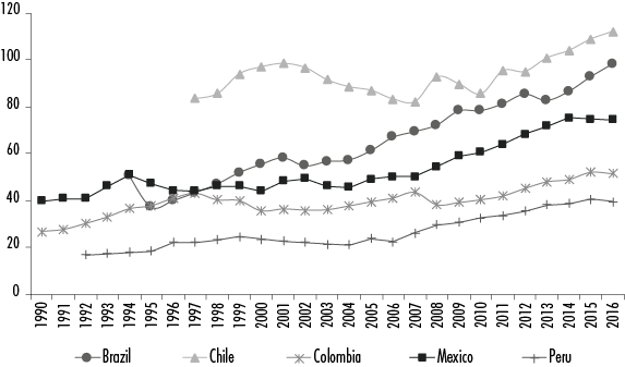
Notes: The indicators of monetary aggregates were M3 for Chile and Colombia, M4for Mexico and Brazil, and liquidity for Peru. Source: calculated by the authors based on information from the International Financial Statistics Yearbook, IMF eLibrary, 2008 and 2018 https://www.elibrary.imf.org/subject/041).
Figure 1 Monetary aggregates to GDP
Another important indicator of financial complexity is the ratios of total credits to GDP. These are not very high in the region except for Chile and Brazil, followed by Colombia as a distant third, and Mexico occupying the last place (Banks of International Settlement [BIS] does not provide data from Peru, see Table 2). This ratio increased throughout the twenty-first century, with the exception of Argentina as explained by the high credit ratios after the convertibility regime’s collapse and the economic crisis in 2001. With the exception of Chile, there was a reduction in the ratio of bank loans to the private sector in early 2000s. This increased during the period after the crisis, but in a reduced manner. This makes it possible to argue that the relationship between foreign capital and the supply of bank loans to the non-financial private sector is not very robust (see Table 2). Thus, with the exception of Chile, credits do not play an important role in the economic evolution of the region’s countries. This would indicate that external flows are not linked to the private sector’s financing.
Table 2 Loans to the non-financial sector, % of GDP
| Argentina | Brazil | Chile | Colombia | Mexico | |
| Credits to the non-financial sector | |||||
| 2000-2007 | 125.8 | 115.9 | 116.5 | 80.8 | 44.9 |
| 2008-2014 | 69.0 | 125.2 | 127.7 | 84.7 | 60.4 |
| 2015-201 9 | 90.8 | 154.3 | 170.9 | 111.7 | 77.4 |
| Credits to the non-financial private sector | |||||
| 2000-2007 | 33.1 | 48.4 | 101.2 | 43.8 | 25.0 |
| 2008-2014 | 19.0 | 63.4 | 115.2 | 50.5 | 32.2 |
| 2015-201 9 | 19.9 | 72.9 | 145.2 | 63.3 | 41.7 |
| Credits bank to the non-financial private sector | |||||
| 2000-2007 | 13.4 | 32.4 | 60.0 | 23.4 | 10.3 |
| 2008-2014 | 13.5 | 56.7 | 73.4 | 36.1 | 15.4 |
| 2015-201 9 | 14.1 | 62.7 | 82.7 | 46.4 | 19.1 |
| Credits to corporations from the non-financial sector | |||||
| 2000-2007 | 29.0 | 34.8 | 73.1 | 32.1 | 15.0 |
| 2008-2014 | 13.6 | 39.5 | 80.3 | 30.3 | 18.4 |
| 2015-201 9 | 13.7 | 44.0 | 101.2 | 36.6 | 25.8 |
Source: created by the authors base on BIS (2020), total credits to the non-financial sector, principal debt (https://www.bis.org/statistics/totcredit.htm?m=26692020).
Another important element of financial complexity is the evolution of the stock market (see Table 3). It evolves inverse to the flow of external capital due to large foreign companies’ reduced share of local capital markets. In other words, these institutions do not participate in their host markets, just as large Latin American companies have a reduced share of local markets.
Tabla 3 Relevant capital market indicators
| Average per period | ||||
| 2000-2007 | 2008-2014 | 2015-2019 | 2000-2019 | |
| Argentina* | ||||
| Listed domestic companies | 108.0 | 100.1 | 94.0 | 102.6 |
| Capitalization of listed domestic companies (% GDP) | 20.4 | 10.8 | 12.7 | 15.4 |
| Stocks traded, total value with regard to (% GDP) | 2.2 | 0.5 | 0.8 | 1.3 |
| Shares traded. turnover of domestic shares (%) | 11.6 | 5.1 | 5.2 | 8.0 |
| Brazil | ||||
| Listed domestic companies | 385.9 | 365.0 | 339.3 | 365.9 |
| Capitalization of listed domestic companies (% GDP) | 49.9 | 51.1 | 38.6 | 48.5 |
| Stocks traded, total value with regard to (% GDP) | 19.2 | 34.1 | 28.6 | 26.6 |
| Shares traded. turnover of domestic shares (%) | 36.8 | 70.2 | 75.4 | 56.2 |
| Chile | ||||
| Listed domestic companies | 244.9 | 229.3 | 216.3 | 231.1 |
| Capitalization of listed domestic companies (% GDP) | 100.9 | 110.4 | 89.8 | 102.7 |
| Stocks traded, total value with regard to (% GDP) | 12.6 | 18.1 | 10.5 | 14.4 |
| Shares traded. turnover of domestic shares (%) | 11.8 | 16.6 | 11.5 | 13.6 |
| Colombia | ||||
| Listed domestic companies | 100.1 | 79.6 | 68.0 | 84.7 |
| Capitalization of listed domestic companies (% GDP) | 39.4 | 56.0 | 35.3 | 47.4 |
| Stocks traded, total value with regard to (% GDP) | 3.8 | 7.2 | 4.3 | 5.2 |
| Shares traded. turnover of domestic shares (%) | 21.2 | 13.2 | 12.4 | 14.9 |
| Mexico | ||||
| Listed domestic companies | 152.6 | 131.1 | 138.0 | 141.6 |
| Capitalization of listed domestic companies (% GDP) | 23.4 | 37.0 | 34.4 | 30.6 |
| Stocks traded, total value with regard to (% GDP) | 6.4 | 9.7 | 9.6 | 8.2 |
| Shares traded. turnover of domestic shares (%) | 27.8 | 26.8 | 27.9 | 27.5 |
| Peru | ||||
| Empresas domésticas listadas | 196.0 | 204.9 | 215.7 | 202.8 |
| Capitalización de las empresas domésticas listadas (% PIB) | 31.8 | 48.7 | 39.7 | 39.7 |
| Acciones comercializadas, valor total respecto al PIB (% PIB) | 3.2 | 2.4 | 1.6 | 2.6 |
| Acciones comercializadas, rotación de las acciones domésticas (%) | 10.0 | 5.3 | 3.7 | 7.1 |
Souce: calculated by the authors based on World Bank data (2020).
The largest number of listed companies is in Brazil, followed by Chile and Peru (a relatively small economy), and then Mexico and Argentina. In terms of capitalization value relative to GDP, Chile tops the list, followed by Brazil and Colombia. Peru is a distant second, followed by Mexico and Argentina.
The behavior of the Mexican Stock Exchange is representative as Mexico is an economy with a lot of multinational and multilatina companies, both in the financial and non-financial sector, with few companies listed in the stock market, and reduced capitalization and turnover ratios, except for Chile.
Finally, we analyze the bond market. The first sign is that the issuance of international bonds has a long history in the region. In the 1970s and 1980s, the countries with the highest volumes of international bond issuance were Mexico, due to the presence of oil and the subsequent large external debt, followed by Brazil. Argentina joined the issuance of international bonds in the 1980s. This trend accelerated in 1990, as explained by the convertibility regime; and Mexico’s and Brazil’s shares drops, Mexico’s due to the signing of NAFTA and Brazil’s to the vitality of the domestic financial market. The issuance of Chilean and Peruvian international bonds is revitalized in the 1990s, continuing until the 2010s. Even in the latter period, these economies lead the issuance of international bonds with respect to their GDP (see Figure 2a).
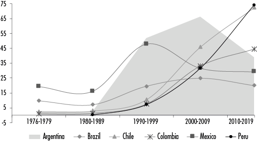
Source: calculated by the authors based on BIS (2020), Table 3 (https://www.bis.org/statistics/secstats.htm?m=2615).
Figure 2a Total international bonds issued by country
The novelty is that, according to the type of issuer, Non-Financial Corporations (NFC) became quite active in issuing international bonds in the twenty-first century, with the exception of Argentina and Brazil (see Figure 2b). The Chilean NFCs have a share of more than 60% of total international bonds issued, reaching in the first and second decade of the 21st century, 30.6% and 46% of GDP, respectively. Mexican NFCs doubled their share between the first and second decades of the 21st century (9% to 19% of GDP) and something similar happened in Peru when it went from 1% to 18% of GDP. An additional element is that most bonds issued are long-term, both from general government as well as from financial and non-financial corporations.
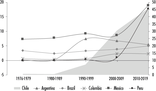
Source: calculated by the authors based on BIS (2020), Table 3 (https://www.bis.org/statistics/secstats.htm?m=2615).
Figure 2b Total international bonds issued by non-financial corporations
The issuance of domestic bonds (see Table 4) indicates that this market became active quite late, with Brazil placing first in the region during the first two decades of the 21st century, with 164% and 311% of the output, respectively (the total includes those issued by the Central Bank). In a distant second place are Mexico and Chile, with significant increases in Colombia and Peru. This indicates that these economies also made progress in developing the domestic bond markets but to a much lesser degree.
Table 4 Domestic bonds issued, % GDP
| Total | General Gov | FC | NFC | ||
| Argentina | 2000-2009 | 7.4 | 2.9 | 4.6 | |
| 2010-2019 | 47.3 | 39.9 | 7.5 | ||
| Brazil | 2000-2009 | 161.4 | 120.0 | 35.5 | 5.9 |
| 2010-2019 | 311.2 | 207.1 | 85.5 | 18.6 | |
| Chile | 2000-2009* | 32.4 | 4.5 | 18.3 | 9.6 |
| 2010-2019 | 99.1 | 24.2 | 50.3 | 24.6 | |
| Colombia | 2000-2009 | 28.3 | 27.9 | 0.5 | |
| 2010-2019 | 89.5 | 87.6 | 0.0 | ||
| Mexico | 2000-2009 | 43.1 | 26.3 | 12.4 | 4.5 |
| 2010-2019 | 95.3 | 59.6 | 28.1 | 7.5 | |
| Peru | 2000-2009 | 15.8 | 5.7 | 6.7 | 3.4 |
| 2010-2019 | 62.8 | 35.1 | 20.0 | 7.8 |
Notes: FC: Financial Corporations, NFC: Non-Financial Corporations; * in recent editions of BIS no domestic bond information is provided; statistics were obtained from previous years and only cover
2008-2015.
In Brazil, the government and financial corporations are the largest issuers of domestic bonds, with NFCs only accounting for a relatively small number of them. Between 2010 and 2014 in Chile (information is only available for the period of 2008-2014) financial institutions are the ones that issued the majority of domestic bonds while NFCs show significant growth. This number though is much lower when compared to the issuance of international bonds. In Mexico, the general government is the one that issued the majority of domestic bonds, with financial corporations accounting for a significant amount while NFCs’ share is insignificant. Finally, the distribution in Peru is relatively the same as that in Mexico, in spite of it being a much smaller and less developed country in the financial sector.
We also analyze the evolution of economies’ external debt (see Table 5). The common denominator in the countries analyzed is that each country’s external debt to GDP is higher in the 2001-2008 stage; it falls significantly in the phase of excess liquidity (revaluation of the exchange rate and low interest rates) and rises again in the period of monetary normalization (2015-2018). This is explained by strong currency depreciations in the region due to the increase in the United States’ interest rate.
Table 5 Evolution if debt to GDP
| Total external debt | Public- guaranteed | Private - unguaranteed | |
| Argentina | |||
| 2000-2007 | 81.3 | 47.1 | 15.2 |
| 2008-2014 | 30.7 | 16.0 | 8.7 |
| 2015-2019 | 38.6 | 19.0 | 8.0 |
| Brazil | |||
| 2000-2007 | 31.8 | 13.5 | 12.7 |
| 2008-2014 | 17.7 | 5.1 | 10.5 |
| 2015-2019 | 27.8 | 9.1 | 15.6 |
| Chile* | |||
| 2000-2007 | 45.9 | 4.3 | 34.9 |
| 2008-2014 | 44.6 | 2.9 | 32.0 |
| 2015-2019 | 64.7 | 6.4 | 47.6 |
| Colombia | |||
| 2000-2007 | 31.1 | 19.2 | 8.4 |
| 2008-2014 | 23.0 | 13.6 | 6.3 |
| 2015-2019 | 40.9 | 24.3 | 12.0 |
| Mexico | |||
| 2000-2007 | 20.3 | 12.8 | 4.8 |
| 2008-2014 | 26.0 | 15.0 | 5.8 |
| 2015-2019 | 37.7 | 24.0 | 8.3 |
| Perú | |||
| 2000-2007 | 45.4 | 32.8 | 7.2 |
| 2008-2014 | 30.3 | 12.2 | 13.6 |
| 2015-201 9 | 33.4 | 9.4 | 19.5 |
Notes: *debts from Banks or non-bank financial institutions are not included; public debt only consists general government and banking, private sector debt includes companies and FDI.
Source: World Bank (2020) (https://data.worldbank.org/) and Central Bnak of Chile (2020) (https://www.bcentral.cl/web/banco-central/areas/estadisticas).
In Argentina, Brazil, Chile and Peru, external debt carries greater weight, especially in the first two stages. Argentina, at the beginning of the new century, has the largest volume of external debt, explained by the crisis it faced between 1999-2001 with the public sector accounting for almost half and the private sector only accounting for a small part. This came about due to the default of public debt in 2001 (which is restructured in 2005) along with a low share of private sector debt. We must point out that after the GFC-2008, the external debt in Argentina is drastically reduced, especially public debt and, to a lesser degree, private debt. It maintained that same composition during the 2015-2018 stage. Brazil is an interesting case that has relatively lower debt than Argentina, although the private sector accounts for a large part of it, especially during 2015-2018, since a good part of the public debt is of domestic origin. This phenomenon also applies to Chile and Peru which have debt greater than Brazil and where the private sector is an important source of external debt. In Colombia and Mexico, external debt is relatively high.
The different behavior of external debt is due to crises (Argentina) and to the fact that the private sector prefers to borrow from the international market as it is cheaper than local markets. This does not happen in Mexico and Colombia, given that there is large capital dissociated from the domestic private sector.
4. EXTERNAL CAPITAL AND ITS EFFECTS: CAPITAL INFLOWS, FINANCING AND GROWTH
In this section we present an econometric analysis to show the causality and effect of these capital flows (FDI and FPI) on financial and real sector variables, as regards a sample of Latin American countries. Specifically, we analyze the relationship between capital inflows and the domestic financial market’s deepening, as well as economic growth and external debt. This is achieved by using non-financial sector’s credit and stock market indicators
Some analyses support the positive effect of FDI and economic growth: neoliberal approaches; those of the new economic geography; the advantages of cluster economies in productivity and technology transfer (Blomström, 1989; Dunning and Lundan, 2008; Wan, 2010). Based on this theoretical approach, recent econometric analyses show the positive effect of FDI on economic growth; an example is the case of the Mexican economy (see Rivas and Puebla, 2016) or the case of Latin America (see Varela and Salazar, 2021). However, there is no difference between periods analyzed and the effects of portfolio investment on financial and real variables are not verified.
This section presents an econometric test to isolate the effect of FDI and portfolio investment on financial and real sector variables and determine their effects in two periods during 2000-2018.
The statistical analysis uses variables obtained from the World Bank database (in millions of dollars at current prices) and the BIS,5 and is divided into two stages. The first corresponds to 2001-2009, starting after the dotcom crisis and ending with the housing crisis. The second covers 2009-2018, and includes the period of quantitative easing and monetary policy normalization from 2014 to 2015, which generated a recessionary process for Latin American economies until 2018.
The variables were filtered using panel unit root tests,6 resulting in first order integration. As such, we used them in logarithmic first difference, meaning the model’s coefficients can be interpreted as growth rates (semi-elasticities). A preliminary inspection of the variables is shown in Table 6, where the average growth rates and the variation coefficient for the two periods analyzed are presented.
Table 6 Average growth rate and variation coefficients for the model´s variables
| 2000-2009 (%) | Var. Coeff | 2009-2018 (%) | Var. Coeff | |
| DGDP | 8.1 | 1.43 | 3.3 | 3.55 |
| DDCPSBanks | 2.9 | 2.98 | 3.4 | 1.33 |
| DMC | 17.9 | 2.12 | 5.3 | 5.63 |
| DTDS | 3.9 | 0.18 | 8.7 | 0.90 |
| DTO | 3.9 | 9.52 | -5.2 | -5.63 |
| DFDI | 9.6 | 4.25 | -0.6 | -67.39 |
| Dcart | 22.0 | 5.33 | 1.6 | -21.84 |
| DS | 16.8 | 3.11 | 0.1 | 17.99 |
| DIDIT | 5.9 | 2.08 | 13.1 | 0.82 |
| DIDIG | 5.8 | 3.62 | 8.5 | 1.69 |
| DIDIF | 8.0 | 5.14 | 20.9 | 1.38 |
| DIDNF | 9.6 | 2.86 | 21.9 | 0.97 |
Notes: DDCPSBanks=growth rate of domestic credit granted by Banks to the private sector; DMC=growth rate of the domestic campanies share capitalization; DGFCF=growth rate of gross fixed capital formation; DTDS= stock debt growth rate; DGCF=Growth rate of gross capital formation; DTO=turnover growth rate; DS=growth rate of traded stocks; DGDP=GDP growth rate; Dcart= portfolio capital inflow growth rate; DFDI= FDI growth rate; Dinflows=growth rate of capital inflows (FDI+Portfolio); DIDIT=growth rate for debt issued by financial institutions in external markets; DIDIG=growth rate for government issued debt in external markets; DIDIF=growth rate for debt issued by financial institutions in external markets; DIDINF=growth rate for debt issued by non-financial institutions in external markets; (1) It should be noted that due to lack of information in this period, the particular effect of portfolio investment could not the statistical tests corresponding to the model chosen, it was concluded that pool is the best type of model. However, as it has auntocorrelation and heteroscedasticity problems, the coefficients will be estimated using the standard corrected errors method assuming first-orden correlation and heteroscedasticity.
Source: created by the authors using data from the World Bank (2020) (https://data.worldbank.org) y BIS (2020) (https://www.bis.org/statistics/secstats.htm?m=2615).
The period of 2009-2018 stands out in the analysis of Table 6. During that time, the growth rate for the turnover (DTO), traded stocks (DS) and GDP growth rate (DGDP) sees a significant reduction compared to the previous period (from 8.1% in 2001-2009 to 3.3% in 2009-2018); commercial bank credit to the private sector (DDCPSBanks) sees modest growth, while foreign currency bond-debt issuance grows vigorously, doubling the average growth rate of foreign currency debt issued by financial and non-financial institutions (20.9% and 21.9%, respectively). Likewise, the average growth rate of external debt stock doubled (from 3.9% in 2000-2009 to 8.7% in 2009-2018). Finally, during 2009-2018, the growth rate of capital inflows decreased, presenting great volatility (variation coefficients for FDI -IFDI- and portfolio capital -Dcart- was -67.39 and -21.84, respectively). In other words, the second period was characterized by greater volatility, less growth, and growing external debt, led by large non-financial companies listing bonds.
After the statistical analysis, using the econometric methodology, we seek to highlight the particular effect of capital inflows (FDI and FPI) on financial and real sector variables in two stages: the first, covers the period of 2001-2009 (with a dummy representing the crisis); the second covers the period of 2009-2018. Next, we will briefly present the coefficients for the different estimates in Table 7 for the proposed periods.7
Table 7 Panel estimation: Panel Corrected Standard Error method (CPSE)
| Dependent Variable | First period (2000-2009) | Second period (2009-2018) | ||||||||||
| Model 1: Explicative variables | Model 1: Explicative variables | Model 2: Explicative variables | ||||||||||
| Constant | DFDI | Crisis | Constant | DFDI | Crisis | Constant | Dcart | Crisis | ||||
| DGDP | Coefficient | 0.036 | 0.012 | -0.044 | Coefficient | 0.034 | 0.010 | -0.052 | Coefficient | 0.036 | 0.003 | -0.079 |
| P-value | 0.000 | 0.072 | 0.000 | P-value | 0.000 | 0.041 | 0.000 | P-value | 0.000 | 0.204 | 0.000 | |
| DDCPSBanks | Coefficient | 0.029 | -0.007 | -0.041 | Coefficient | 0.035 | 0.026 | -0.019 | Coefficient | 0.039 | -0.009 | -0.009 |
| P-value | 0.257 | 0.816 | 0.450 | P-value | 0.000 | 0.056 | 0.423 | P-value | 0.000 | 0.089 | 0.790 | |
| DMC | Coefficient | 0.087 | 0.242 | 0.592 | Coefficient | -0.010 | 0.047 | 0.659 | Coefficient | -0.012 | 0.125 | 0.448 |
| P-value | 0.543 | 0.340 | 0.142 | P-value | 0.857 | 0.634 | 0.002 | P-value | 0.831 | 0.007 | 0.002 | |
| DTDS | Coefficient | 0.029 | 0.044 | 0.051 | Coefficient | 0.088 | 0.048 | -0.028 | Coefficient | 0.097 | 0.028 | -0.082 |
| P-value | 0.167 | 0.167 | 0.312 | P-value | 0.000 | 0.056 | 0.572 | P-value | 0.000 | 0.016 | 0.066 | |
| DTO | Coefficient | -0.005 | 0.237 | -0.472 | Coefficient | 0.001 | 0.007 | -0.528 | Coefficient | 0.004 | 0.035 | -0.421 |
| P-value | 0.927 | 0.065 | 0.002 | P-value | 0.960 | 0.950 | 0.000 | P-value | 0.906 | 0.369 | 0.003 | |
| DS | Coefficient | 0.056 | 0.651 | 0.302 | Coefficient | -0.003 | -0.008 | 0.028 | Coefficient | -0.005 | 0.151 | -0.018 |
| P-value | 0.688 | 0.001 | 0.398 | P-value | 0.973 | 0.949 | 0.910 | P-value | 0.939 | 0.003 | 0.922 | |
| DIDIT | Coefficient | 0.029 | 0.016 | 0.240 | Coefficient | 0.122 | 0.044 | 0.057 | Coefficient | 0.140 | 0.057 | -0.030 |
| P-value | 0.284 | 0.663 | 0.000 | P-value | 0.000 | 0.125 | 0.364 | P-value | 0.000 | 0.000 | 0.516 | |
| DIDIG | Coefficient | 0.058 | -0.019 | 0.048 | Coefficient | 0.091 | 0.035 | -0.054 | Coefficient | 0.102 | 0.041 | -0.274 |
| P-value | 0.143 | 0.769 | 0.595 | P-value | 0.001 | 0.400 | 0.388 | P-value | 0.000 | 0.084 | 0.029 | |
| DIDIF | Coefficient | 0.040 | 0.052 | 0.321 | Coefficient | 0.198 | 0.092 | 0.085 | Coefficient | 0.239 | 0.126 | 0.110 |
| P-value | 0.264 | 0.566 | 0.006 | P-value | 0.005 | 0.277 | 0.644 | P-value | 0.000 | 0.001 | 0.354 | |
| DIDINF | Coefficient | 0.053 | -0.092 | 0.424 | Coefficient | 0.177 | 0.085 | 0.277 | Coefficient | 0.204 | 0.072 | 0.055 |
| P-value | 0.415 | 0.418 | 0.009 | P-value | 0.002 | 0.084 | 0.006 | P-value | 0.000 | 0.001 | 0.204 | |
Notes: DDCPSBanks=growth rates for domestic credit provided by private sector banks; DMC=growth rate for domestic companies share capitalization; DTD=stock debt growth rate; DTO=turnover growth rate; DS=traded stocks growth rate; DGDP=GDP growth rate; Dcart=portfolio inflow growth rate; DFDI=FDI growth rate; Dinflow=growth rate of capitol inflows (FDI+ Portfolio); DIDIT=growth rate for debt issued in external markets; DIDIG=growth rate for government issued debt in external markets; DIDIF=growth rate for debt issued by financial institutions in external markets; DIDINF=growth rate for debt issued by nonfinancial institutions in external markets. Source: created by the authors using data from the World Bank (2020) (https://data.worldbank.org) and BIS (2020) (https://www.bis.orgistatistics/secstats.htn?2615).
Table 7 shows the coefficients of the two models in two periods; the exogenous or explanatory variables are the FDI growth rate (DFDI) and the portfolio capital growth rate (DFPI). It should be noted that due to lack of information in the first period, the effect of portfolio investment on the variables analyzed could not be obtained (observations were lost in the process of logarithmic linearization and differentiation). A dummy, which was not significant, was included for the period of 2015 onwards.8 As a result, it can be said that the volatility present in the second period analyzed was a feature characteristic of the period after the 2008-2009 crisis.
The following can be stated based on an analysis of Table 7.9
First period. The FDI growth rate stands out as having a positive effect with regards to GDP growth and share turnover (with a 90% level of certainty for these two variables), as well as with regards to shares traded (with 99% certainty, see Table 7). The effect of the crisis is captured by the dummy through the GDP growth rate’s negative and significant ratio, share turnover and the growth of debt through the issuance of bonds (see Table 7).
Second period.i)The FDI growth rate has a positive effect on GDP (95% certainty), domestic private credit and external debt (90% certainty);ii)the portfolio investment growth rate (DFPI) positively affects that of the capitalization of domestic shares, traded shares (99% certainty) and external indebtedness (95% certainty, see Table 7). It should be noted that FDI (DFDI) also has a positive effect on the growth of non-financial institutions’ debt placement in international markets (90% certainty); its ratio is even higher than in the case of GDP (0.08 vs. 0.01).
We ascertain that the FDI to GDP ratio drops from the first to the second period and the relevant feature is that FDI (DFDI) and portfolio investment (DFPI) positively affect the growth rate of external indebtedness (DTDS). In the second period, portfolio investment boosts the stock market (which can be seen in the DMC and DS coefficients, ‘0.125’ and ‘1.151’ respectively). Unlike the first period, FDI did not promote this market’s growth (the ratios are not significant), and even the ratio of FDI to the DTDS level was higher than that of bank credit to the private sector (DDCPSBanks) (0.048 vs. 0.026, respectively). We also see that portfolio investment energized the foreign currency bond market, mainly that of financial and non-financial institutions (0.12% and 0.07%, respectively).
With these findings we can claim that the different forms of development for large domestic (multilatina) and transnational companies in Latin American countries affected the stock market’s vitality through FDI (specifically via mergers and acquisitions), with a reduced impact on economic growth. One can also see that after the GFC-2008, FPI had an important role in invigorating financial markets, both the bond and stock market, although with a reduced effect on economic growth (the average growth rate of FPI and FDI plummeted in the second period (see Table 6)). Furthermore, the inflow of capital did not increase economic growth, nor did bank financing to the private sector. Based on the aforementioned, we can say that capital investment opened up a new form of external debt, specifically through the non-private business sector, that is to say via large companies.
Thus, one of the main effects of decoupling large companies’ activities from domestic financial and productive markets is reflected in the promotion of continuous indebtedness due to placing their debt abroad and their expansion into external markets. When you add to this the fact that much of FDI comes in the form of mergers and acquisitions, it has little impact on accumulation and prolongs economic stagnation, income concentration and dependence on external capital. This creates conditions for growing financial instability for all economies in the region.
5. CONCLUSIONS
Within the heterodox approach, credits - and financing in general - are not necessarily related to production as there is a variety of explanations for financial risk. Keynes (1936) explains financial instability from the present view of future variations in the interest rate which, combined with institutional investors’ speculative activity, generates gains or losses within the space of capital circulation. Kalecki (1971) relates financial risk to companies’ balance sheets, thereby assuming a mix of productive and financial activities that can reduce losses if investment prospects are not met. Minsky (1975) tries to merge Keynes’ (1936) and Kalecki’s (1971) approaches by proposing a business cycle where investment spending generates increasing leverage rates that modify interest rates and the volume of bank loans. Minsky’s approach concludes by arriving at an explanation where the business cycle is linked to movement of capital and how the main agents of economies develop, specifically corporations and the government.
By applying this analysis to the behavior of some Latin American economies, we found that the institutional change that took place in the 1990s and opened the Latin American financial markets to the rest of the world failed to revolutionize the behavior of the main financial institutions. It created a great liquidity of international funds with a reduced deepening of financial institutions. However, this happened without strongly expanding credit’s share of financing as large companies led a great development in the issuance of bonds in the international space. This in turn promoted a growing external indebtedness where the private sector played an important role. Even in the Brazilian economy, where the domestic bond market developed strongly, NFCs do not take on a very active role.
From the econometric analysis we can conclude that during the first decade of the 21st century, the FDI growth rate had a positive effect on GDP, mainly on the turnover rate of the stock market, traded stocks and the listing of debt-bonds by non-financial institutions. However, in the 2010s, after the GFC-2008, the effect of the FDI growth rate on GDP declined. It should be noted that FDI had a greater effect on external debt than on growth. The growth rate of portfolio investment positively affects the growth rate of domestic share capitalization, traded stocks, external borrowing and bond issuance for all institutions, but especially for financial and non-financial ones. That is to say, portfolio investment became a rejuvenating agent for the capital and bond market in the second period, leading to greater external indebtedness.
We can therefore affirm that one of the main effects of decoupling large companies’ activities from domestic financial markets is reflected in the continuous indebtedness by placing debt externally. This, together with the entry of FDI in the form of mergers and acquisitions, ends up reducing accumulation, prolongs economic stagnation and promotes income concentration.
ACKNOWLEDGMENTS
The authors would like to thank the anonymous peer reviewers’ comments which contributed to improving the quality of this work.
REFERENCES
Berle, A. y G. Means (1932). The modern corporation and private property.Transaction Publishers. [ Links ]
Blomström, M. (1989). Foreign investment and spillovers. Routledge. https://doi.org/10.4324/9781315774671. [ Links ]
Dunning, J. H. y Lundan, S. M. (2008). Multinational enterprises and the global economy. Edward Elgar Publishing. [ Links ]
Fama, E. (1991). Efficient capital markets: II. The Journal of Finance, 46(5). https://doi.org/10.2307/2325486. [ Links ]
Kalecki, M. (1954). Theory of economic dynamics. George Allen and Unwin Ltd. [ Links ]
______(1971). Selected essays on the dynamics of the capitalist economy. 1933-1970. Cambridge University Press. [ Links ]
Keynes, J. M. (1919). The economic consequences of the peace. Cambridge University Press. [ Links ]
______(1930). The treatise on money. Vol. II. Cambridge University Press. [ Links ]
______(1936). The general theory of employment, interest and money. Harcourt. [ Links ]
Luxemburgo, R. (1913). The accumulation of capital. http://www.marxists.org/archive/luxemburg/1913/accumulation-capital/index.htm. [ Links ]
Minsky, H. (1975). John Maynard Keynes. Macmillan Press Ltd. [ Links ]
______(1986). Stabilizing and unstable economy. McGraw-Hill. [ Links ]
Modigliani, F. y Miller, M. (1958). The cost of capital, corporation finance and the theory of investment. The American Economic Review, 48(3).https://www.jstor.org/stable/1809766. [ Links ]
Mott, T. (2010). Kalecki'sprinciple of increasing risk and Keynesian economics. Routledge. [ Links ]
Pierre-Manigar, M. (2009). El plan de convertibilidad en Argentina: límites a la política monetaria. Ola financiera. http://www.olafinanciera.unam.mx/new_web/04/pdfs/Pierre-OlaFin-4.pdf. [ Links ]
Polanyi, K. (1944). The great transformation: the political and economic origins of our time. Farrar and Rinehart. [ Links ]
Rivas, S. y Puebla, A. (2016). Inversión Extranjera Directa y crecimiento económico. Revista Mexicana de Economía y Finanzas, 2(11 ).http://www.scielo.org.mx/scielo.php?script=sci_arttext&pid=S1665-53462016000200051. [ Links ]
Seccareccia, M. (2003). Pricing, investment and the financing of production within the framework of the monetary circuit: some preliminary evidence. En L. Rochon (ed.). Modern theories of money (pp. 173-197). Edward Elgar. [ Links ]
Shiller, R. (2000). Irrational exuberance. Princeton University Press. [ Links ]
Steindl, J. (1945). Small and big business. Economic problem of the size of the firms. Basil Blackwell. [ Links ]
Stiglitz, J. (1988). Why financial structure matters. Journal of Economics Perspectives, 2(4). https://doi.org/10.1257/jep.2.4.121. [ Links ]
Toporowski, J. (2000). The end of finance, capital market inflation, financial derivatives and pension fund capitalism. Routledge. [ Links ]
______(2018). Michael Kalecki: An intellectual biography, By intellect alone 1930-1970. Volume II. Palgrave Macmillan. [ Links ]
Varela, M. y Salazar, G. (2021). Foreign direct investment in Latin America: effects on growth and development. En N. Levy, J. Bustamante y L-Ph. Rochon (coords.). Capital movements and corporation dominance in Latin America: reduced growth and increased instability (pp. 158-173). Edward Elgar. [ Links ]
Wan, X. (2010). A literature review on the relationship between foreign direct investment an economic growth. International Business Research, 3(1). https://doi.org/10.5539/ibr.v3n1p52. [ Links ]
1 Berle and Means (1932) argued that the financial practices which replaced shareholder’s pre-emptive rights (which ensure the sharing of current profits and the companies’ future income power) with vested rights bestowed great power to those in control as it allowed them to distribute profits and property rights according to their own interests.
2Return on assets is determined by quasi profits (q), minus the costs of storage (c) plus the liquidity premium (l) (Keynes, 1936, chap. 17).
3 Keynes, inThe Treatise on Money,1930, vol. II, chap. 37), offers a different explanation. Using Riefler’s statistical work for the United States, he points out that the interest rate set by the Central Bank has a strong influence on short and long-term interest rates. This means that the Central Bank is capable of influencing the whole interest rate structure, a fair strategy in times of crisis.
4M4measures money in general which represents all sectors’ liabilities minus the financial sector. It is money and securities issued by the central government and non-financial corporations’ deposits. M1 is all fully liquid circulating money (International Financial Statistics Year Book, 2007, IMF eLibrary, https://www.elibrary.imf.org/subject/041).
5Due to lack of information, Argentina was not included. This means that the statistical analysis was carried out using Brazil, Chile, Colombia, Mexico and Peru. It should be noted that the GDP was analyzed in constant dollars for 2010 and had the same behavior in the estimates.
6Stationarity tests were performed for variables at logarithmic levels (Fisher, Im-Pesaran-Shin and Levin-Lin-Chin tests). It was concluded that the variables have unit roots in levels and are stationary in first logarithmic difference (as such, they will be interpreted asquasielasticities), see annexed stata files (https://bit.ly/2ZnvLvJ).
7After performing the statistical tests corresponding to the model chosen, it was concluded that the best model is pool. However, when presenting problems of autocorrelation and heteroscedasticity, the coefficients will be estimated using the method of standard errors corrected assuming first-order correlation and heteroscedasticity.
9We include the link to the stata .do file, as well as the file with model information, in order to allow for a more detailed review (http://bit.ly/2ZnvLvJ).
Received: May 25, 2021; Accepted: November 03, 2021
 Este es un artículo publicado en acceso abierto bajo una licencia Creative Commons
