1. INTRODUCTION

The literature on wages and employment shows that economic shocks affect the behavior of labor markets, making it difficult for businesses to acquire the labor force they need and for the economically active population to find job opportunities in line with their expectations. Matching theory studies exactly this macroeconomic outcome of interactions between various agents in markets where frictions prevent instantaneous adjustments to the level of economic activity (^{Álvarez de Toledo et al., 2008}). According to ^{Mortensen and Pissarides (1994}), the volatility inherent in these difficulties is actually what drives loss and creation of employment.

For ^{Mendes et al. (2010}), the level of matching in the labor market is a function of productive affinity; that is, the productivity of businesses partly determines the affinity of the workers they seek, although information asymmetries may hinder the process. Similarly, ^{Pissarides (2000}) finds that, when random shocks are present in the economy, a matching function (MF) of the labor market is a good alternative for estimating the expected income of both businesses and workers.

These studies give indications that the MF, understood as a mathematical relation describing the formation of mutually beneficial relationships between agents, is a valuable tool for analyzing the flows into and out of unemployment resulting from these agents’ decisions. The analysis of flows derived from MFs is facilitated by the development of agent-based models (ABM), which, supported by simulations, expose the dynamics, interactions, and behavioral patterns of these flows.

ABMs are composed of agents with characteristics that make them unique, autonomous, and capable of interacting with each other and with their environment, with the aim of explicitly representing social or natural phenomena without having to rely on mathematical tractability (^{Railsback and Grimm, 2012}). This type of model makes it possible to reproduce patterns observed in reality. For example, ^{Lewkovicz et al. (2009}) observed that in France there was a high rate of unemployment in workers over 50 years of age, and, using an ABM, found that this pattern was caused by the imposition of a new model of labor contract.

On the other hand, complex systems are composed of heterogeneous and rationally constrained individuals who decide on their actions and strategies in response to the very outcome of their interaction with each other (^{Arthur, 2013}). Since the 2008 crisis financial crisis, when the dominant models had few positive contributions to policy design, there was a growing interest in incorporating elements of complexity theory (^{Battiston et al., 2016}). Complexity theory allows the innovation and social transformation processes to be studied, through agent-based computational models sufficiently flexible to articulate the micro- and macro-levels of the economy (^{Richiardi, 2017}).

Working within this approach, ^{Hamill and Gilbert (2016}) propose an ABM that presents the performance of a labor market where workers are differentiated according to age and skills, and have to choose between continuing in their job or quitting to look for a new one. The model also adopts some socioeconomic indicators that characterized the town of Guildford, capital of the county of Surrey in the UK, during the period from 2009 to 2013 (this reference model will be referred to as ABM-REF). The authors find that heterogeneity in wages complicates the matching process, potentially leading the economy into severe unemployment.

The research so far presented, including that of ^{Hamill and Gilbert (2016}), share a peculiarity: workers may remain indefinitely unemployed if they are not matched to any vacancy. The above scenario could be plausible in economies that ensure compensatory supports to the lack of labor income, but it does not seem feasible in developing economies where there are no social security or unemployment insurance provision mechanisms in place. This could be the case for 58.8% of the world's economies (International Labor Organization [ILO], ²⁰¹⁸).

This reality increases the probability that the population will venture into entrepreneurial activities (depending on economic need and business management capacity), with self-employment predominating, predictably. The ILO (2018) points out that self-employment is a popular source of occupation in countries that do not have unemployment benefits, where it reaches 37.4% of the labor force, while in countries with some form of social security it barely represents 15.5%.

Given the difficulty of generalizing matching results such as those presented above to the context of developing countries, the present article reviews the implications of relaxing the ^{Hamill and Gilbert (2016}) ABM assumption that the worker can choose to remain indefinitely unemployed. This is achieved by including the option of self-employment as an occupational activity. It is predicted that incorporating this option will result in lower permanence in unemployment for workers and, under certain conditions, in lower long-term unemployment.

This result would be consistent with the findings of ^{Glocker and Steiner (2007}) who, using a pseudo-panel data analysis for Germany, find a positive relationship between the time that workers are unemployed and the rate of entry into self-employment. The authors point out that this effect is significant compared to that of other possible determinants such as age or professional qualifications, and that it offsets the negative effect that prolonged unemployment can have on credit constraints and individual expectations.

Likewise, the results would be consistent with those obtained by ^{Thurik et al. (2008}), who through a vector autoregressive model estimate the dynamic interrelation between unemployment and self-employment for a panel of countries belonging to the Organization for Economic Cooperation and Development (OECD) for the period 1974-2002, finding that high unemployment rates induce more people to become entrepreneurs (refuge effect); however, the decision to become an entrepreneur reduces unemployment at the macroeconomic level. The results suggest that the refuge effect is relatively small, meaning that a policy to encourage innovative and high-growth entrepreneurship could have more favorable results than one aimed at inducing the unemployed to enter self-employment.

Studies such as ^{Fonseca et al. (2001}) seek to integrate self-employment into MFs, focusing on the effect of entry costs to self-employment on employment levels. The authors introduce a factor of innate entrepreneurship in individuals. Meanwhile, ^{Narita (2020}) studies the effects of public policies on informality on the composition of the labor market, using an MF whereby a choice is made between working and entrepreneurship in both the formal and informal sectors.

Unlike the aforementioned studies in which the choice of entrepreneurship is associated with probabilities exogenous to the worker, the present article introduces the option of self-employment governed by a matching process between vacancies and workers, where the selection of the worker depends on an analysis of the opportunity cost of entrepreneurship in relation to forgoing the possibility of earning a wage. In this sense, the choice is underpinned by the worker's perception of the labor market and is therefore endogenous (^{Berkhout et al., 2016}).

This paper consists of five sections, including this introduction. The second section provides an overview of the ABM-REF. In the third section, the self-employment component is integrated into the aforementioned model to subsequently analyze its effect on the inflows and outflows of unemployment in the labor market. In the fourth section, the simulation exercise is developed with the self-employment extension. The fifth section presents the results of the extended model and its comparison with the reference model, as well as some implications for developing economies. Finally, the sixth section offers some conclusions and recommendations for future research.

2. ^{HAMILL AND GILBERT'S (2016}) AGENT-BASED MODEL (ABM-REF)

This section presents an overview of the ABM-REF, which illustrates the basic dynamics of the flows between unemployment, employment, and inactivity in the Guildford labor market. It should be noted that the ABM-REF is based on an MF, whereby the amount of work actually performed in the economy depends on the arrangements linking job-seeking workers to available jobs in the labor market. In this function, the incentive for businesses to match is the generation of output through the labor force, while, workers, on the other hand, are motivated to match by the incentive of a wage (^{Pissarides, 2000}).

3. INCORPORATING THE OPTION OF SELF-EMPLOYMENT IN THE LABOR MARKET

Integrating the self-employment option for workers into the ABM-REF allows us to analyze the effect of this occupational opportunity on flows into and out of unemployment. Unlike ^{Narita (2020}), who simulates a labor market where the probability of entrepreneurship depends on experience, the extension proposed here is based on the availability of vacancies and the wage offered, in line with ^{Berkhout et al. (2016}),²⁵ where unemployed workers choose between seeking employment or entrepreneurship, relying on what is called the "propensity indicator for self-employment as an economic activity."²⁶ G(μ _w , 𝜎 _w , k _w ) This indicator is understood as an approximation to the probability of starting up, as a function of the mean (μ), the standard deviation (σ), and the bias (k), of the wage set (w) offered by the businesses in which the worker could be employed. Thus, μ _w , σ _w and k _w represent, respectively, in terms of wages, the mean to which the worker can aspire, the volatility, and the asymmetry of the distribution.

On the other hand, maintaining equality between the number of workers and the number of jobs available in the economy (which for the ABM-AMP corresponds to salaried jobs and self-employment) requires monitoring the enterprises created. Otherwise, the AMB-REF’s underlying assumption, the economy starts from an initial state where all workers and jobs are occupied, cannot be guaranteed, and, therefore, the ABM-AMP would not provide unemployment inflows and outflows based on observable statistics. To maintain the aforementioned equality and make the matching functions equivalent, we limit the number of self-employment opportunities to 130, setting wage jobs at 870 (consistent with the evidence presented by ^{Hamill and Gilbert (2016}) for Guildford, which indicates that 13% of the labor force engaged in self-employment activities, over the period 2009-2013).²⁷

Earnings from self-employment are calculated using individual labor productivity obtained through an allocation process based on a log-normal distribution, similar to that used to allocate wages. These earnings can be equal to or greater than the wage sought from employment. On the other hand, self-employment ventures will close when the following occurs: the entrepreneur retires (upon reaching the age of 60),²⁸ or the earnings are less than their minimum acceptable wage, in which case they will become unemployed and may seek another job or try to start up again. If the enterprise closes, the individual becomes unemployed. ^{Douglas and Shepherd (2000}) understand that considering skill differences in employment options makes economic sense, although, unlike these authors, the AMB-AMP is oriented towards the pecuniary implications of the matching process and the choice of self-employment.²⁹

Figure 1 presents the processes described above, both for the ABM-REF and the ABM-AMP, highlighting with a dotted rectangle the contribution of the proposed incorporation of the inflows and outflows of self-employment. These processes are described below.

Mechanics of exit from unemployment. In the ABM-REF, the unemployed can only exit this status through matching with a vacancy. However, incorporating self-employment provides an additional choice for the unemployed person, who must now choose between self-employment or continuing the job search. The worker's decision depends on the propensity to start up. The assumption behind this approach is that the worker can only engage in one productive activity each quarter as a result of an optimal choice process.

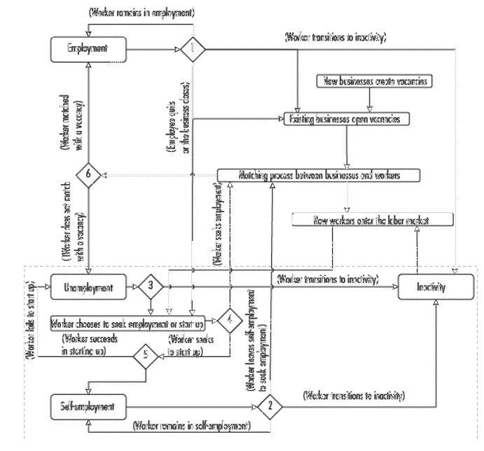
Source: Compiled by the authors based on ^{Hamill and Gilbert (2016}). The numbering inside the diamonds suggests the sequence of the model. Unified Modeling Language (UML) was used. For further explanation of this language, see http://openaccess.uoc.edu/webapps/o2/bitstream/10609/9121/1/Intro_UML.pdf

Figure 1 ABM-AMP Labor Market Model 

Mechanics of entry and exit from self-employment. In the first instance, each unemployed person is shown to be familiar with their environment and characteristics, represented by the dispersion measures μ _w , 𝜎 _w , and K _w , based on the wages of the vacancies for which they are eligible.³⁰ Via these measures, the worker can gauge their propensity to start up a productive activity, G(μ _w , 𝜎 _w , k _w ) . This propensity consists of three components, one for each dispersion measure, resulting from logistic functions, such that the results can be equivalent to those of ^{Berkhout et al. (2016}). The propensity to choose self-employment as an economic activity has a negative relation with the average wage observed by a worker. The component associated with the mean (Cμ) is given by:

Likewise, the propensity to start up has a positive relationship with the standard deviation, which represents the uncertainty that exists in the labor market about wages offered. Thus, the higher the standard deviation,³¹ the less certain the worker is about the possibility of receiving a wage higher than or equal to the average. The standard deviation weighting is specified as

Finally, the bias has a negative effect on the propensity to self-employment in the sense, given that it is caused by vacancies with high wages, then finding a job with above-average pay is more likely. But the opposite can also occur, lower-than-average wages skew the distribution and, therefore, entrepreneurship has a lower associated opportunity cost. This component (c _k ) is defined as:

Since we do not have information on the relative importance of each component of the propensity to start up (G), we decided to add them together and give them a uniform weight, represented as G=13Cμ+Cσ+Ck.. ³²The threshold of the indicator above which self-employment is chosen is based on the midpoint of its range. Thus, those unemployed who obtain G<12 are workers in search of work, while those who obtain G≥12 are workers seeking to start up.³³ However, as already mentioned, there are a limited number of self-employment opportunities in the market, and this number may be lower than the number of people seeking to become entrepreneurs.

In this sense, the workers who finally enter self-employment in each period are chosen randomly, which allows for the inclusion of workers of any salary range. In each period, the worker's minimum acceptable wage is compared with the wage from self-employment. If the latter is lower than the former, the worker moves from self-employment to unemployment. Those who are classified as workers seeking to become self-employed remain unemployed as long as they do not succeed, and may also opt to seek employment.

4. THE SIMULATION EXERCISE

To allow comparison between models and thus validate the extension, it was necessary to run both in a controlled simulation environment under careful parameterization. The ABM-AMP comparison was simulated with NetLogo, which is the program used in the reference model. The parameters controlled in the simulations are wage flexibility and the percentage of workers moving to inactivity or quitting their jobs; this allowed for calibration of the extension, making the two models technically comparable. As for wage flexibility, the maximum increase is 5%, without considering the possibility of decreases. Additionally, the percentage of employed and unemployed that transits to inactivity each quarter is 2% and 15%, respectively.

The analysis is strengthened via the incorporation of the scenarios used by ^{Hamill and Gilbert (2016}) regarding the rate of workers quitting their jobs each quarter, ranging from 1% to 5%, are presented for both models. Table 1 presents the ABM-REF results for the mean (μ) and the standard deviation (σ) ³⁴ of the simulated flows for each of the relevant indicators. It can be seen that, with a mean of 6.0%, the simulation that comes closest to the observed mean of 6.1% is the one that considers a resignation rate of 1%.

Table 1 Means and standard deviations [μ(σ) ] of the AMB-REF for different resignation rates 

		Quitting rate (%)
		1	2	3	4	5
Indicator (%)	UEF	18.14 (0.92)	19.91 (0.89)	21.9 (0.99)	23.04 (1.14)	24.63 (1.28)
	Unemployment rate	5.98 (0.35)	5.84 (0.29)	5.49 (0.38)	5.49 (0.21)	5.46 (0.32)
	Long-term unemployment	23.46 (1.17)	21.77 (1.19)	20.16 (1.08)	18.98 (1.32)	17.91 (1.30)

Source: Taken from ^{Hamill y Gilbert (2016}). Standard deviation is shown in parentheses.

Similarly, Table 2 presents the results of the ABM-AMP, where it can be seen that the 5% resignation rate generates an unemployment rate very similar to that observed in the reference period. This is the first element of validation that the extension is more representative of reality, in that it produces findings consistent with the empirical evidence.

Table 2 Means and standart derivations [μ(σ) ] of the AMB-AMP for different resignation rates 

		Tasa de renuncia (%)
		1	2	3	4	5
Indicator (%)	UEF	15.92 (0.80)	17.39 (0.87)	18.32 (0.66)	19.45 (0.92)	20.92 (0.99)
	Unemployment rate	6.46 (0.32)	6.45 (0.36)	6.30 (0.35)	6.21 (0.30)	6.10 (0.41)
	Long-term unemployment	24.23 (0.97)	23.24 (1.14)	22.66 (0.85)	22.20 (1.36)	21.06 (0.98)

Source: Compiled by the authors. The standard derivation is shown in parentheses.

An inverse relationship can be observed between the average unemployment rates in Tables 1 and 2 as the resignation rate increases. This is because the higher the number of unemployed workers, the higher the outflow, as more jobs are freed up and there is more interest in filling them. When there is a low resignation rate, outflows are reduced and unemployment increases.

The second element of validation concerns the stability of the simulated unemployment rates, which were analyzed for 100 periods.³⁵ According to ^{Hamill and Gilbert (2016}), this rate ranged between 5.2% and 6.6% during their analysis. Figure 2 presents the evolution of this rate in the case of the ABM-AMP for different quitting rates (see Table 2). The criterion for choosing the most appropriate simulation to represent an economy such as Guildford's is that the mean of the simulated unemployment rate should be close to the observed rate, while the variations should remain within its range. It is found that the scenario that best complies with the above is where 5% of workers quit their jobs.³⁶

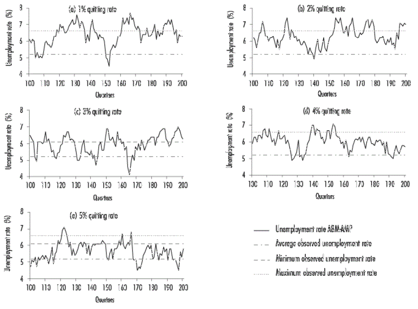
Source: Compiled by the authors using NetLogo.

Figure 2 Quarterly unemployment rate for different quitting rates in the ABM-AMP. 

The variations observed in Figure 2 are due to the pressure generated by the mechanics of entry into self-employment on the efficiency of the matching between vacancies and unemployed. The average unemployment rate obtained in the ABM-AMP, with the aforementioned indicators, was 6.1%. This rate is similar to that observed in the South East of England between 2009 and 2013. Figure 2e shows that the quarterly unemployment rate obtained by the ABM-AMP oscillates in the range observed in the period (5.2%-6.6%), which means that incorporating self-employment mechanics to the ABM-REF, in line with ^{Berkhout et al. (2016}) is appropriate for the analysis.

5. RESULTS

First, the results and implications of the incorporation of the self-employment option in the flows between unemployment and employment are presented, comparing the results with those of the reference model. The findings related to the flows between unemployment and self-employment are described. Second, the effects of the self-employment option on economic indicators of the labor market are presented, such as the wage level and long-term unemployment.

Effects of incorporating self-employment on labor flows

Figure 3a shows the EUF in both models, which seem to oscillate around a medium value; however, the ABM-AMP shows higher volatility than the ABM-REF. These flows consist of people who quit their jobs and those who lose their jobs due to external shocks, in relation to the total number of workers in the economy.

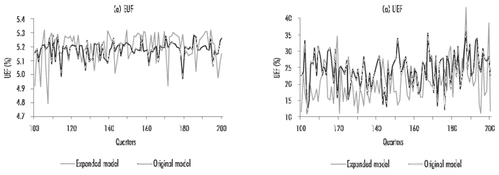
Source: Compiled by the authors using NetLogo.

Figure 3 Comparison of flows between unemployment and employment 

This figure shows that the EDFs of the models do not show large differences. This is because the exit parameters are the same in both: 5% of workers quit their jobs and then look for a new one, and 2% of small businesses with up to two employees (including self-employment, when applicable) close each quarter. This could change if the possibility of job search while employed is added to the model, in which case we would expect a decrease in the inflow to unemployment, but also an increase in long-term unemployment, given the competition from unemployed workers.

Although the difference is not visually evident (see Figure 3b), the average EUF in the ABM-AMP is 2% lower than that presented in the ABM-REF. This is because, despite the fact that the matching mechanics were the same in both models (albeit with a distinct number of vacancies-to), the unemployed in the ABM-AMP had an alternative to matching, which reduced the outflow into wage employment.

Figure 4 shows that the number of workers seeking self-employment remains at around 87 per quarter due to the lack of trends in the main labor market indicators. This suggests that the stability of the ABM-AMP has an impact on the number of workers seeking to start up and, in addition, that for some unemployed people, the supply of vacancies does not meet the standards that make the opportunity cost of seeking self-employment lower than that of looking for a job, resulting in a propensity to seeking self-employment, resulting in a high propensity to entrepreneurship G≥12 . Following ^{Berkhout et al. (2016}), the above could represent situations of economic sectors with low vacancy supply or low wages, where seeking to start up becomes more prevalent than seeking employment.

Source: Compiled by the authors.

Figure 4 Workers seeking to start up 

On the other hand, Figure 5 shows that there is a temporal correspondence between workers who move between self-employment and unemployment. This is confirmed by the correlation index between both flows, which is 76%. This is due to the limit of 130 job opportunities, imposed with the objective of maintaining similarity with the number of enterprises observed in Guildford, and the high level of occupancy of these opportunities, which conditions the possibility of new income to the freeing up of spaces.

Note: USF refers to the number of workers moving from unemployment to self-employment, while SUF refers to the workers moving from self-employment to unemployment as a proportion of self-employed workers. Source: Compiled by the authors.

Figure 5 Self-employment inflows and outflows (ABM-AMP) 

Effects of self-employment on wages and long-term unemployment

Figure 5b shows the evolution of the self-employment to unemployment flow (SUF) that occurs when the income associated with self-employment is less than the worker's minimum acceptable wage. This suggests that in the ABM-AMP there are always unemployed people seeking self-employment and taking advantage of entrepreneurship opportunities. Thus, if there were no restrictions on entry into self-employment, a significant part of the labor market might be willing to take up a place in this occupational field.

Figure 6 presents the evolution of long-term unemployment statistics and the wage level of employed workers for both ABM-REF and ABM-AMP. Figure 6a shows that the long-term unemployment ratio in both models oscillates around a mean value of 18.3% in the case of ABM-AMP and 24.1% for ABM-REF, so the average of ABM-AMP is lower (24%) than that of ABM-REF, as expected. This is because, in the long-term, unemployed workers have the possibility of transitioning to self-employment and developing an economic activity for at least one quarter.

Source: Compiled by the authors.

Figure 6 Comparison of long-term unemployment and average wages 

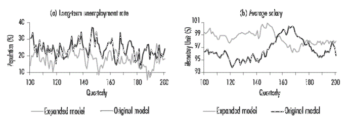
Figure 6b shows the evolution of the average quarterly wage received by employed workers. It should be noted that the ABM-REF only shows the effect of wage flexibility on the labor market, while the extended model includes the effect of the opportunity for self-employment on the labor supply.

It can be seen that the average wage is higher in the expanded scenario for most quarters. Overall, ABM-REF wages are 1.9% lower than ABM-AMP wages. This is because self-employment attracts workers receiving low wages, while those who choose to participate in the labor market are generally workers with higher wages. Consequently, the incorporation of the option of entrepreneurship into the economy increases the average wage. However, between quarters 155 and 176, the ABM-REF average wage was higher, perhaps because of the entry of both businesses with high-wage vacancies in the reference model and low-wage businesses in the ABM-AMP.

6. CONCLUSIONS

Self-employment is a genuine alternative for workers with entrepreneurial ambitions or who find themselves in saturated labor markets. In recent years, governments and international organizations have allocated significant resources to promoting entrepreneurship as a labor option for the population. This policy is informed, in part by a desire to reduce the rigidity of the labor market and guarantee macroeconomic stability. This article has studied the effect of considering the occupational alternative of self-employment on the inflows and outflows of unemployment via the ABM model proposed by ^{Hamill and Gilbert (2016}). The self-employment option was incorporated via the ^{Berkhout et al. (2016}) model, which proposes a choice problem between job search and entrepreneurship that considers the opportunity cost of the alternatives through the calculation of the probability of entrepreneurship.

It was seen that the incorporation of the self-employment option reduces the rate of workers who participated in the matching process. This trend was reflected in the reduced unemployment-to-employment flows. Likewise, the calculation of an individual indicator of propensity to self-employment was incorporated, based on the dispersion of wages offered to workers. The indicator modified the inflows and outflows of unemployment (in relation to the reference model) in a manner consistent with economic theories on the labor market. This finding demonstrates that this indicator can be considered an effective instrument for measuring the preference for a labor option that can be supported by dispersion measures, such as self-employment.

In light of the above, this paper concludes that entrepreneurship is less attractive the greater the ratio between the number of vacancies and unemployed workers, and to the extent that there is a greater supply of vacancies with above-average salaries. The propensity to start up allows us to infer that those who seek to start up in the labor market will prefer to do so in ventures that provide an income higher than the average wage of available vacancies. Conversely, in a highly-volatile labor market with few vacancies per worker and below-average wages (regardless of level), more workers will opt for self-employment. Due to the wage bias, we would expect an increase in the number of low value-added ventures, which would make the search for an income close to the average wage part of a rational decision, given that wages above this level would be unlikely and therefore more difficult to obtain.

For a developing economy facing circumstances such as a low wage level in available jobs and a limited number of vacancies in relation to the number of workers, the population will be more likely to seek self-employment as an option. In public policy terms, this suggests that simply promoting entrepreneurship may be inadequate, as the precarious conditions of the labor market are already a sufficient incentive. Understood in this way, support should be given to existing businesses (including the self-employed) to consolidate and attempt to transition to more robust forms of enterprise and thus increase the number of vacancies available in the market. This could involve, for example, increased support in the form of social security, access to financing, or tax advice.

It is important to emphasize that the extension developed can be used as a basis for integrating other mechanisms considered essential for the practical functioning of an effective labor market, such as wage negotiation, the job search process, learning over time, the effect of job skills, the benefits of self-employment, or the role of entrepreneurship in decision-making. This will allow us to obtain a more comprehensive view of the labor market that includes the different processes that affect the inflows and outflows of unemployment. Likewise, when seeking to understand developing economies, it is crucial to continue to incorporate elements related to labor informality and underemployment into the context of entrepreneurial propensity.

REFERENCES

Aljure, Y. y Gallego, J. A. (2010). Desigualdad y leyes de potencia. Cuadernos de Economía, 29(53 ).https://revistas.unal.edu.co/index.php/ceconomia/article/view/18597/19495. [ Links ]
Álvarez de Toledo, P., Núñez, F. y Usabiaga, C. (2008). La función de emparejamiento en el mercado de trabajo español. Revista de Economía Aplicada, 16(48 ).https://www.redalyc.org/pdf/969/96915830001.pdf. [ Links ]
Arthur, W B. (2013). Complexity economics: A different framework for economic thought. SFI Working Paper 2013-04-012. Santa Fe Institute. https://sfi-edu.s3.amazonaws.com/sfi-edu/production/uploads/sfi-com/dev/uploads/filer/a1/3e/a13e8ad4-cd39-4422-8cc3-86c543699f6d/13-04-012.pdf. [ Links ]
Battiston, S., Farmer, J. D., Flache, A., Garlaschelli, D., Haldane, A. G., Heesterbeek, H.,... y Scheffer, M. (2016). Complexity theory and financial regulation. Science, 351(6275 ). https://doi.org/10.1126/science.aad0299. [ Links ]
Begg, D., Vernasca, G., Fischer, S. y Dornbusch, R. (2014). Economics. McGraw-Hill Education. [ Links ]
Berkhout, P., Hartog, J. y Van Praag, M. (2016). Entrepreneurship and financial incentives of return, risk, and skew. Entrepreneurship: Theory and Practice, 40(2). https://doi.org/10.1111/etap.12219. [ Links ]
Buchanan, M. (2004). Power laws and the new science of complexity management. Strategy and Business, 34. https://www.strategy-business.com/article/04107?pg=all. [ Links ]
Chéron, A. y Rouland, B. (2011). Endogenous job destructions and the distribution of wages. Labour Economics, 18(6). https://doi.org/10.1016/j.labeco.2011.07.005. [ Links ]
Douglas, E. y Shepherd, D. (2000). Entrepreneurship as a utility maximizing response. Journal of Business Venturing, 15(3). https://doi.org/10.1016/ S0883-9026(98)00008-1. [ Links ]
Fonseca, R., Lopez-Garcia, P. y Pissarides, C. (2001). Entrepreneurship, startup costs and employment. European Economic Review, 45(4-6 ). https://doi.org/10.1016/S0014-2921(01)00131-3. [ Links ]
Glocker, D. y Steiner, V. (2007). Self-employment: a way to end unemployment? Empirical evidence from German pseudo-panel data. IZA DP No. 2561. http://ftp.iza.org/dp2561.pdf. [ Links ]
Hamill, L. y Gilbert, N. (2016). Agent-based modelling in economics. Wiley. [ Links ]
Lewkovicz, Z., Domingue, D. y Kant, J. D. (2009). An agent-based simulation of the French labour market: studying age discrimination. The 6th Conference of the European Social Simulation Association. http://www-desir.lip6.fr/~smasite/seminaires/Exposes/ZL_DD_JDK.pdf. [ Links ]
Mendes, R., Van Den Berg, G. y Lindeboom, M. (2010). An empirical assessment of assortative matching in the labor market. Labour Economics, 17(6). https://doi.org/10.1016/j.labeco.2010.05.001. [ Links ]
Mortensen, D. y Pissarides, C. (1994). Job creation and job destruction in the theory of unemployment. Review of Economic Studies, 61(3). https://doi.org/10.2307/2297896. [ Links ]
Narita, R. (2020). Self-employment in developing countries: a search-equilibrium approach. Review of Economic Dynamics, 35. https://doi.org/10.1016/j.red.2019.04.001. [ Links ]
Organización Internacional del Trabajo (OIT) (2018). Paid employment vs. vulnerable employment: A brief study of employment patterns by status in employment. Spotlight on work statistics (No 3 - June 2018). ILOSTAT. https://ilo.org/wcmsp5/groups/public/---dgreports/---stat/documents/ publication/wcms_631497.pdf. [ Links ]
Pissarides, C. (2000). Equilibrium unemployment theory. Cambridge MIT Press. [ Links ]
Railsback, S. y Grimm, V. (2012). Agent-based and individual-based modeling: a practical introduction. Princeton University Press. [ Links ]
Richiardi, M. G. (2017). The future of agent-based modeling. Eastern Economic Journal, 43(2). https://doi.org/10.1057/s41302-016-0075-9. [ Links ]
Thurik, A., Carree, M., Stel, A. y Audretsh, D. (2008). Does self-employment reduce unemployment? Journal of Business Venturing, 23(6). http://dx.doi.org/10.1016/j.jbusvent.2008.01.007. [ Links ]
2Without this flexibility, matching would be more difficult and the analysis could generate higher unemployment rates than actually exist.
3In analytical terms, a power law is a functional relationship between two quantities A and B, whereby A is proportional to B raised to a power n. One of these quantities can even be the frequency of the other, resulting in a random variable reaching high values with a low probability and low values with a high probability. Power laws reflect a pattern of organization that is characteristic of complex systems (Buchanan, 2004). Pareto's income distribution law, according to which 20% of the population concentrates 80% of the wealth, is a basic example of a power law (Aljure and Gallego, 2010).
4Thus, if two vacancies pay the same, they are considered equal regardless of whether they are offered by different companies.
5The flows are relative; that is, they express the number of people who change their labor status from one period to another in percentage terms. In all cases the base refers to the initial period.
6This study contributes to the ABM-AMP, as it considers the processes of entry and exit to unemployment in a labor market in which self-employment is an option.
8To maintain the possibility of matching, Hamill and Gilbert (2016) propose that these workers are employed by companies with two jobs. In the present study, these are transformed into effective self-employed.
9Although an entrepreneur could continue working after reaching this age, this assumption is made to ensure consistency with the ABM-REF.
10In any event the comparison of results is not appropriate given the differences between the respective methodologies used in each study.
14When there are less than three vacancies, the indicator is set at 2/3, which is consistent with what is observed in labor markets with limited labor supply.
15These terms should not be confused with w and w, which refer exclusively to the propensity to start up.
16Similar to Hamill and Gilbert (2016), 200 periods were simulated, although, for obtaining valid indicators only the last 100 were taken into account; the rest were considered part of the experimentation necessary to stabilize the simulation.
17The effect on unemployment of resignation rates of 6% and above was also analyzed. The test yielded unemployment levels higher than the peaks observed in Guildford, so these rates were discarded from the analysis.
18Given that the model does not distinguish between formal and informal markets, nor does it consider the formalities (legal or illegal) associated with self-employment or the costs of contracting companies.
Received: January 14, 2021; Accepted: August 04, 2021
Este es un artículo publicado en acceso abierto bajo una licencia Creative Commons