


 nueva página del texto (beta)
 Inglés (pdf)
 Artículo en XML
 Referencias del artículo
 Enviar artículo por email
 Citado por SciELO
  Similares en
SciELO
Similares en
SciELO 
 Permalink
INTRODUCTION
Leukemia is a blood disease distinguished by the ab- normal production of white blood cells [1]. Its diagnosis uses a blood smear where the presence of myeloblasts or lymphoblasts is determined [2] [3]. This examination is usually a time-consuming manual process and requires microscopist expertise [4] [5] [6]. Recently, image processing techniques with machine learning have been used, which integrate image processing and segmentation, feature extraction and selection, and a classification algorithm [7] [8]. The most critical steps are segmentation and selection of significant features [9] [10] [11].
During microscopic analysis, cells are stained to provide visibility and contrast [12]. The segmentation stage separates the cells from the rest of the image from the acquired color. Among the techniques that have been applied to segment are K means [13] [14] [15] [16] [17] [18], Fuzzy c-means [19], Triangle thresholding [20] [21] [22], and Otsu thresholding [9] [23] [24] [25] [26], which are usually accompanied by the Watershed algorithm to divide adjacent or overlapping cells [27] [28].
From the nucleus or cytoplasm, parameters are calculated that help to identify cancer types. Several features can be analyzed, including geometric, statistical, and texture [21] [26] [29]. The number of parameters used should be limited using a reduction algorithm to improve the efficiency of classification model [30] [31].
Some methods to decrease the number of characteristics are Univariate feature selection (k-Best) [32], Social Spider Optimization Algorithm (SSOA) [33], Genetic Algorithm (GA) [25], Statistically Enhanced Salp Swarm Algorithm (SESSA) [34], Linear Discriminant Analysis (LDA) [35] and Principal Component Analysis (PCA) [35] [36] [37]. The latter is a statistical technique that reduces the dimension of a data set and generates a new set of uncorrelated variables. These are called principal components (PC), and their relationship preserves the maximum variation from the original data set [38] [39].
On the other hand, color models are used to define the way to represent the tones mathematically. The color spaces RGB [9] [26], CMYK [16] [20] [35], HSI [23] [40], HSV [19] [24], and CIE L*a*b [14] [41], and grayscale [25] [42] [43] have been used for this type of application. Studies have identified that RGB is not ideal for the segmentation of these cells, while HSI, HSV, and CMY perform better [44] [45]. In a group of images where the capture brightness effect varies, the use of HSV space may be the most appropriate because it separates the image intensity from the color information [17] [19].
In feature extraction, statistical and color properties have been obtained from various spaces such as, RGB [21] [30], HSV [13] [19] [46], HSI [35] and CIE L*a*b [14]. Of these, RGB and HSV spaces are the most widely used, but the use of these representations has not been justified [14] [21] [33] [47]. Although statistical and color features are an important source of information, no studies have yet been performed to compare the accuracy of color space using these characteristics in cell sorting with staining.
This paper proposes to use a principal component analysis with statistical descriptors as input variables to determine the color space that best represents the information of a set of images. This process is analyzed by using the k nearest neighbors (kNN) algorithm and a confusion matrix to determine the accuracy of the predictive model. The objective of the study is to propose a tool to image processing methodologies to identify the model that best represents the content of the region of interest (ROI). In particular, it is applied to identify two types of cancer, acute lymphoid leukemia (ALL) and multiple myeloma (MM).
MATERIAL AND METHODS
Image Dataset Definition
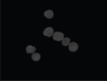
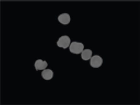
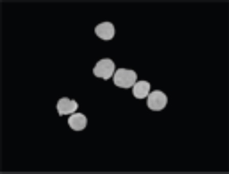
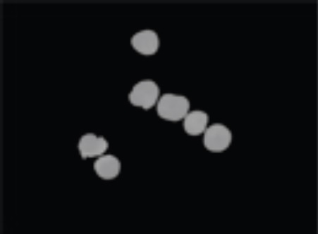
The set of images used in this work is a collection of microscopic bone marrow images of patients diagnosed with B-lineage acute lymphoid leukemia and multiple myeloma, published in The Cancer Imaging Archive (TCIA) by Gupta, A. and Gupta, R. [48]. They have a resolution of 2560x1920 pixels, were captured using a Nikon Eclipse-200 microscope at 1000x magnification, and slides were stained with Jenner-Giemsa stain. This study used 60 samples, 30 ALL and 30 MM.
Nucleus Segmentation of Leukemia Cells
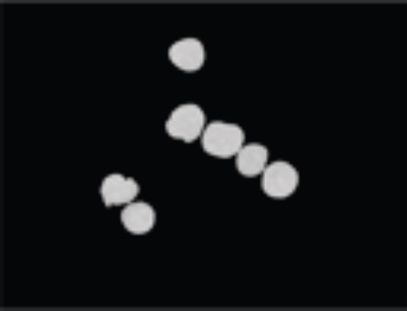
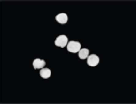
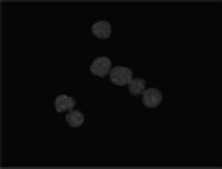
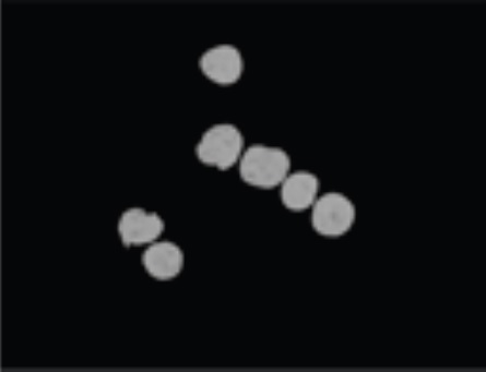
Based on studies by Jagadev and Virani [17], Mirmohammadi et al. [19], and Rahman and Hasan [21], the image segmentation was performed using the HSV space, considering that it separates the intensity of the image from the color information, and the images of the database do not have uniform brightness. For the segmentation process, first, the intensity of the images was adjusted to a range of 0.1 to 0.7 using the value channel (V) to decrease the capture luminance effect [19]. The ROI was defined with a threshold value in the Hue (H) and Saturation (S) components. After a binary segmentation, the holes were filled using a morphological closure with disk shape structure element of radius 4 [49]. The watershed algorithm was used to the resulting image to separate the overlapping nuclei. Subsequently, objects with an area of fewer than 17500 pixels and elements with an eccentricity greater than 0.80 and solidity less than 0.65 were removed [14] [21] [50]. The ROI was established from the original images using the binary mask. A total of 484 blast cell nuclei, 168 ALL and 316 MM, were then extracted. The segmentation results for two sample images are visualized in Figure 1.

Figure 1 Steps of Leukemic Cell Segmentation. ALL original image is shown in a). ALL Image enhancement in b). ALL binary mask in c). ALL filtering and watershed segmentation in d). ALL segmentation result in e). MM original image in f). MM Image enhancement in g). MM binary mask in h). MM filtering and watershed segmentation in i). MM segmentation result j).
Feature Extraction
Mean, variance, standard deviation, skewness, kurtosis, entropy, and energy, were calculated for each nucleus from an image for each color space channel and grayscale. Equations 1 to 7 show the definition of each one of these parameters, where Z represents the intensity as a random variable, p(Zi), i= 0, 1, 2, ..., L-1 is the probability of occurrence of the value Zi and L is the number of different possible values [51]. For each leukemia cell, a total of 21 features were obtained in each color space and 7 for grayscale.
Feature Selection
The most significant features of each color space were identified using principal component analysis. First, the number of statistical descriptors in the dataset was reduced using the “statistics” and “FactoRMine” libraries of Rstudio software [52] [53]. For this, we first checked for a low partial correlation value between each pair of features, using the Kaiser-Meyer-Olkin (KMO) coefficient. If for any of these pairs, mean-variance, mean-standard deviation, mean-skewness, etc., the KMO coefficient is less than 0.5, the value indicates that it is not appropriate to use PCA in that model. Then Bartlett's test of sphericity (BTS) with a significance level of p<0.05 is used to estimate the correlation between variables.
PCA for each color model was performed based on an initial data table represented by a matrix of 484 rows, containing 168 observations of ALL and 316 MM type cells. The measurement result for each statistical descriptor is shown by columns (21 characteristics for the RGB, CMY, HSV, HSI, and CIE L *a*b color spaces and 7 for grayscale). Table 1 shows an example of this for the RGB model components.
Table 1 Data matrix for RGB for an example image. Mean (M), variance (V), standard deviation (SD), Skewness (S), energy (Er) and entropy (Et). The initial of RGB channels was added to each descriptor.
| Sample | MR | VR | SDR | SR | KR | ErR | EtR | MG | … | EtG | MB | … | EtB |
|---|---|---|---|---|---|---|---|---|---|---|---|---|---|
| ALL_1_1 | 85.26 | 266.19 | 16.32 | -0.22 | 0.71 | 0.02 | 0.74 | 42.10 | … | 0.59 | 103.07 | … | 0.62 |
| ALL_1_2 | 85.09 | 253.95 | 15.94 | -0.48 | 0.07 | 0.02 | 0.74 | 42.70 | … | 0.59 | 105.67 | … | 0.63 |
| ALL_1_3 | 88.99 | 69.71 | 8.35 | 0.31 | 0.13 | 0.03 | 0.63 | 42.63 | … | 0.56 | 106.09 | … | 0.55 |
| ⁝ | … | …… | … | … | … | … | … | … | … | … | … | … | ⁝ |
| ⁝ | … | … | … | … | … | … | … | … | … | … | … | … | ⁝ |
| MM_30_10 | 143.32 | 99.41 | 9.97 | 1.33 | 3.03 | 0.03 | 0.65 | 65.77 | … | 0.65 | 120.03 | … | 0.52 |
| MM_30_11 | 97.95 | 337.36 | 18.37 | 0.93 | 2.23 | 0.02 | 0.77 | 43.93 | … | 0.60 | 106.36 | … | 0.61 |
| MM_30_12 | 122.91 | 138.44 | 11.77 | 0.42 | 0.08 | 0.02 | 0.70 | 57.04 | … | 0.67 | 115.60 | … | 0.54 |
Each table column is standardized to an average of 0 and a standard deviation of 1 using Equation 8, where Xj is the value to be standardized, Xjs represents the standardized value and, µx and σx are the average and the standard deviation of the column.
A covariance matrix was calculated using the standardized values for each table to estimate the correlation and dependence between variables. Equation 9 was used to evaluate covariances between each pair of characteristics. Where σjk is the covariance between the two variables, Xj and Xk represent the standardized value of variables j and k, µj and µk are the column averages of variables j and k, and n is the total data per column. The correlation coefficient of the covariances was determined by Equation 10. It is obtained by dividing the covariance by the standard deviations of Xj and Xk represented by σj and σk.
The covariance matrix C is represented as in Equation 11, where Cov(i, j) is the covariance between the elements in row i and column j. This matrix is decomposed into its eigenvalues and eigenvectors to determine the principal components. By solving Equation 12, the eigenvalues λk are obtained and for each of them, its eigenvector V k is determined using Equation 13, where I is the identity matrix. The eigenvectors correspond to the principal components, and the eigenvalues define the magnitude of the variance of the new set of variables. Finally, the eigenvectors are sorted in descending order to select the components that retain at least 80% of the information from the original data set.
ALL and MM Classification
The ALL and MM cancer types were classified using the principal components or new variables. For this purpose, the k nearest neighbor algorithm was employed using the Rstudio software [54]. Data was randomly divided into two sets. 80% of them were used as training data and the remaining 20% as test data.
In the training phase, the kNN algorithm stores the set of input variables to establish a relationship between them and the conditions to be classified, calculating a distance between the rows of training data and the test set data. It was determined as a function of the Euclidean distance (ED) using Equation 14, where A and B represent the principal component vectors A= (x1, x2, x3, x4, ... xm), B= (y1, y2, y3, y4, ... ym), and m, the dimensionality of the feature space.
The resulting vector was ordered from smallest to largest so that the smallest distance is considered the k nearest neighbor.
Subsequently, a number for k was defined to determine the nearest neighbors to include in the voting process using Equation 15. N represents the total data in the training set. The operation resulted in a k = 17.
Finally, to determine the performance of the kNN classifier, the confusion matrix was applied. The metric provided is the accuracy and is defined by Equation 16. Where TP is the true positives, FN is the false negatives, FP indicates the number of false positives, and TN is the number of true negatives.
Statistical Analysis
Lastly, differences of accuracy between color and grayscale spaces were analyzed using a one-way analysis of variance (ANOVA) and Tukey's posthoc test. The sample size was calculated using statistical power analysis. A significance level of 0.05 was established, with a power of 0.8 and an effect size of 0.25. The study determined a sample size of 35. The normality of the residuals was assessed by performing the Shapiro Wilks test, and Bartlett's test demonstrated the homogeneity of variances. For each analysis, was used a significance level of p<0.05.
RESULTS AND DISCUSSION
This section shows the results of the comparison between color spaces and grayscale. Table 2 shows an example of channel decomposition and grayscale conversion of an example image.
Table 2 Channel division of color representations. Channel 1, Channel 2 and Channel 3 correspond to the color band of each color space.
| Color System | Channel 1 | Channel 2 | Channel 3 |
|---|---|---|---|
| Grayscale |
|
||
| RGB |

|

|
|
| CMY |
|

|
|
| HSI |
|
 |
 |
| CIE L*a*b |

|
|
|
| HSV |

|
 |
 |
As presented in Table 1, KMO coefficient was calculated; in all cases, the value was greater than 0.5. Bartlett's test was performed considering the parameters of all images as input, presenting for each color space a significant p-value less than α = 0.05. Thus, the application of the PCA is adequate. The results of these tests are shown in Table 3.
Table 3 Results for Kaiser-Meyer-Olkin measure of sampling adequacy (KMO) and Bartlett’s test of sphericity (BTS). Chi-square (χ²), degrees of freedom (df), p value (p), statistic (stat) and grayscale (GS).
| Test | Stat | GS | RGB | CMY | HSI | L*a*b | HSV |
|---|---|---|---|---|---|---|---|
| KMO | 0.61 | 0.72 | 0.72 | 0.68 | 0.71 | 0.62 | |
| χ² | 5779 | 20621 | 20621 | 20728 | 20133 | 18346 | |
| BTS | df | 21 | 210 | 210 | 210 | 210 | 210 |
| p | <0.05 | <0.05 | <0.05 | <0.05 | <0.05 | <0.05 |
The summary of the PCA is shown in Table 4. The principal components were selected according to the total variance method, retaining at least 80% of the information of the original set of variables. In RGB, CMY, CIE L*a*b, and HSI spaces, 4 PCs were taken; in HSV, 5 PCs; and in grayscale, 2 PCs.
Table 4 Principal component analysis summary. The percentage of cumulative variance (Cum. Var) retained by the PC's are highlighted in blue. Principal component (PC), eigenvalue (λ), variance (Var).
| Color System | PC | λ | Var (%) | Cum. Var (%) |
|---|---|---|---|---|
| Grayscale | 1 | 3.49 | 49.9 | 49.9 |
| 2 | 2.73 | 38.9 | 88.8 | |
| RGB | 1 | 8.02 | 38.2 | 38.2 |
| 2 | 5.95 | 28.3 | 66.5 | |
| 3 | 1.72 | 8.21 | 74.7 | |
| 4 | 1.46 | 6.94 | 81.7 | |
| CMY | 1 | 8.02 | 38.2 | 38.2 |
| 2 | 5.95 | 28.3 | 66.5 | |
| 3 | 1.72 | 8.21 | 74.7 | |
| 4 | 1.46 | 6.94 | 81.7 | |
| HSI | 1 | 6.42 | 30.6 | 30.6 |
| 2 | 5.18 | 24.7 | 55.2 | |
| 3 | 4.00 | 19 | 74.3 | |
| 4 | 1.85 | 8.82 | 83.1 | |
| CIE | 1 | 7.53 | 35.9 | 35.9 |
| 2 | 6.00 | 28.6 | 64.5 | |
| 3 | 2.04 | 9.71 | 74.2 | |
| 4 | 1.49 | 7.11 | 81.3 | |
| HSV | 1 | 5.82 | 27.7 | 27.7 |
| 2 | 4.51 | 21.5 | 49.2 | |
| 3 | 3.11 | 14.8 | 64.0 | |
| 4 | 1.96 | 9.36 | 73.3 | |
| 5 | 1.83 | 8.71 | 82.0 |
The results show that grayscale retains more information in its first two components than the color spaces (see Table 4 data highlighted in blue). The CIE L*a*b space has the highest information loss of 81.3%.
A two-dimensional PCA space was projected for each color model considering the first two components with the highest contribution, as shown in Figure 2. The upper and right coordinates (abscissa and ordinate axis for PC1 and PC2 loadings) show the degree of contribution to the principal components. In these graphs, the black vectors called loadings represent the statistical descriptors. Charge vectors range is from -1 to 1. Charges close to |1| indicate that the variable strongly influences the principal component; those close to 0 denote a weak influence.

Figure 2 PCA biplot for components 1 and 2. Grayscale is shown in a), RGB in b), CMY in c), HSI in d), CIE L*a*b in e), and HSV in f). Ellipses represent a concentration of the scores for each group set with 95% confidence boundaries. Mean (M), variance (V), standard deviation (SD), Skewness (S), energy (Er) and entropy (Et).
A coefficient greater than |0.5| is considered significant to define a PC. For example, for Figure 1a corresponding to grayscale PCA, the mean (M), skewness (S), kurtosis (K), and energy (Er) contribute most to PC1. Variance (V), standard deviation (SD), energy (Er) and entropy (Et) contribute most to PC2.
The angle between loadings is their correlation. Vectors with equal directions are positively correlated, and those with opposite directions are negatively correlated. If they present an angle of 90°, there is no correlation. The vertical and horizontal axes show the percentage of variability explained by the principal components. The points on the graph are the channel measurements of the color models. Cancer types are grouped in concentration ellipses, ALL cells in blue and MM cells in orange.
As shown in Figure 2, vector loadings differ between color representations, yet it is possible to establish a reliable prediction model because the loadings are significant. Although the clusters of the two cancers overlap at some points in the two-dimensional PCA space, a clear separation is visualized between the ALL and MM descriptors (Figure 2a to Figure 2f. The precision results when evaluating the predictive model using kNN are shown in Table 5. Each of the 35 samples was studied using a different random data set.
Table 5 kNN Accuracy results for each color model. Data are in percentage. Grayscale (GS). Average (µ).
| No. | GS | RGB | CMY | HSI | L*a*b | HSV |
|---|---|---|---|---|---|---|
| 1 | 86.6 | 89.7 | 89.7 | 87.6 | 95.9 | 92.8 |
| 2 | 87.6 | 91.8 | 91.8 | 93.8 | 100.0 | 92.8 |
| 3 | 86.6 | 90.7 | 90.7 | 84.5 | 93.8 | 86.6 |
| 4 | 85.6 | 89.7 | 89.7 | 86.6 | 95.9 | 86.6 |
| 5 | 88.7 | 95.9 | 95.9 | 93.8 | 96.9 | 93.8 |
| 6 | 84.5 | 93.8 | 93.8 | 88.7 | 97.9 | 89.7 |
| 7 | 84.5 | 88.7 | 88.7 | 80.4 | 96.9 | 86.6 |
| ⁝ | ⁝ | ⁝ | ⁝ | ⁝ | ⁝ | ⁝ |
| 34 | 78.4 | 92.8 | 92.8 | 89.7 | 95.9 | 87.6 |
| 35 | 88.7 | 91.8 | 91.8 | 87.6 | 93.8 | 85.6 |
| µ | 84.7 | 91.8 | 91.8 | 87.9 | 95.5 | 89.4 |
A one-way ANOVA was then applied to compare the performance of each color model statistically. First, the normality of the residuals was tested using the Shapiro-Wilks test; the p-value = 0.0947 showed that they did follow normal behavior. Bartlett's test determined compliance with homogeneity of variance between treatments with a p-value of 0.2215, suggesting no evidence of statistically significant variation between color representations for ANOVA.
The variance analysis revealed a significant difference between the color models with a p-value less than 0.05 (See Table 6).
Table 6 One-way ANOVA results. Sum of squares (SS), mean square (MS).
| Source | Df | SS | MS | F value | p-value |
|---|---|---|---|---|---|
| Model | 5 | 2436 | 487.2 | 54.12 | <2e-16 |
| Error | 204 | 1836 | 9.0 |
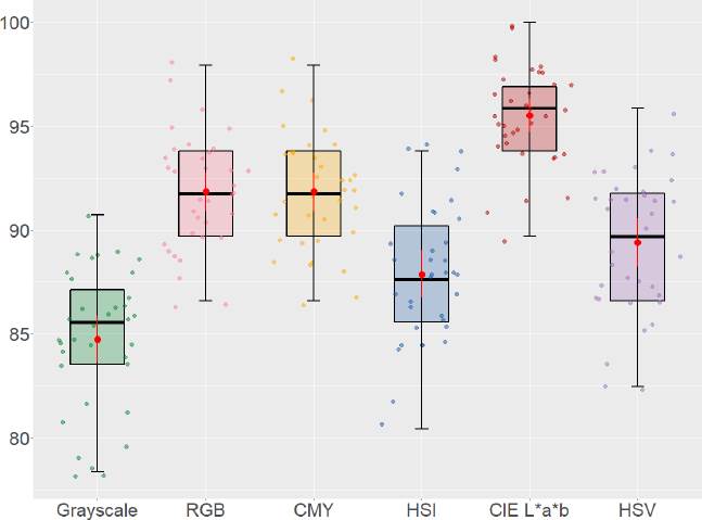
In Figure 3, the distribution of color representations exhibits a normal distribution; outliers are minimal. The whiskers in the box represent the boundaries of the precision samples drawn for each group. The red dot indicates the mean accuracy of color representation. In grayscale was 84.7; in RGB, 91.8; in CMY, 91.8; in HSI, 87.9; in HSV, 89.4; and in CIE L*a*b, 95.5. The predictive model given by the characteristics of the CIE L*a*b color space obtained the highest accuracy, followed by the RGB and CMY spaces. Grayscale was the worst performer.
The pairwise comparisons of means of the color models obtained by Tukey's test can be seen in Figure 4.

Figure 4 Tukey post hoc test pairwise comparison plot. Extended lines in blue color show statistically significant differences between the pairs of means, and extended lines in purple indicate that there is no statistical difference between the means.
In the graph, the extended lines show the 95% confidence intervals. Those crossing the 0 points indicate that there is no statistically significant difference between the pairs of means. The analysis revealed that there is no inequality between RGB and CMY spaces (p-value = 1.00); and HSI and HSV spaces (p-value = 0.27408).
CONCLUSIONS
The use of machine learning and image processing methods play an important role in image analysis for prognosis and early detection of blood cancer. Research for leukemia image classification techniques has used color characteristics from RGB and HSV spaces [21] [30] [13] [19] [46], but other color models are rarely used.
This article presents a methodology to compare the accuracy of different color models to represent the characteristics of leukemia cells. Of the color spaces analyzed, the CIE L*a*b best described the two cancer types, ALL and MM, using color moments with an average accuracy of 95.52%.
Compared to reference articles, the accuracy obtained in this study was superior to that of [36], which used RGB and grayscale space color and texture features. The PCA and the KNN and SVM classifiers were used, obtaining an accuracy of 91.45% and 92.63%, respectively.
Likewise, a better performance was obtained than [30], which used the color characteristics of the RGB space and compared six classifiers; KNN (80.7%), tree classifier (75.8%), ANN (83.5%), logistic regression (82.4%), random forest (81.0%) and SVM (73.6%). The method proposed was similar to the studies [14] [19] in which the SVM classifier was used. In [14], the color characteristics of the RGB, HSV, and CIE L*a*b spaces were used, reaching an accuracy of 95.28%, and in [19], texture characteristics of the grayscale were used, achieving an accuracy of 95%. The presented method has provided novel information on how color spaces can influence the selection of features for image analysis of leukemic cells. Future research could extend the classification approach by considering other cancer types or subtypes, using other classifiers, or selecting different feature selection methods.

