


 nueva página del texto (beta)
 Inglés (pdf)
 Artículo en XML
 Referencias del artículo
 Enviar artículo por email
 Citado por SciELO
  Similares en
SciELO
Similares en
SciELO 
 Permalink
INTRODUCTION
The World Health Organization (WHO) states that glaucoma is the second leading cause of blindness in the world, only after cataracts [1]. Since there is no cure for glaucoma [2], it is necessary to diagnose this disease early to delay its development [3].
Glaucoma is characterized by optic nerve damage due to increased degeneration of nerve fibers [4]. Since symptoms appear until the disease is severe, glaucoma is called a silent thief of sight [5]. Typically, aqueous humor drains out of the eye through the trabecular meshwork, but when the passage is obstructed, aqueous humor accumulates. The increase in this fluid will cause pressure to grow and cause ganglion cell damage [6]. However, it was found that the pressure measurement was not specific or sensitive enough to be the only useful indicator for detecting glaucoma because visual impairment would occur without increasing pressure. Therefore, a comprehensive examination should also include the use of images and visual field tests to analyze the retina [7].
Fundus imaging is the process of obtaining a two-dimensional projection of the retinal tissue employing reflected light. Finally, the resulting 2D image contains the image intensity that indicates the reflected light amount. Color fundus imaging is used to detect disease, where the image has R, G, and B bands, and their intensity changes highlight different parts of the retina [8].
Due to their non-invasiveness, fundoscopy and optical coherence tomography (OCT) has become the imaging methods of choice for the detection and evaluation of glaucoma [9]. Nevertheless, due to its cost, OCT is not readily available.
There are different types of glaucoma, such as open-angle, closed-angle, secondary, normal-tension, pigmentary, and congenital glaucoma [10]. Some types require surgical treatment [11]. The optic disc and cup, peripapillary atrophy, and retinal nerve fiber layer [12] are four structures that are considered essential for detecting glaucoma. Family history has also been shown to be genetically related to the onset of the disease [13].
In most cases, treatment in the early stage of the disease can prevent total vision loss in glaucoma patients [14], so a system that can help ophthalmologists make a diagnosis could increase the chances of saving people's vision. However, designing a system that provides reliable tests for glaucoma diagnosis is a complicated and stimulating task in clinical practice [15].
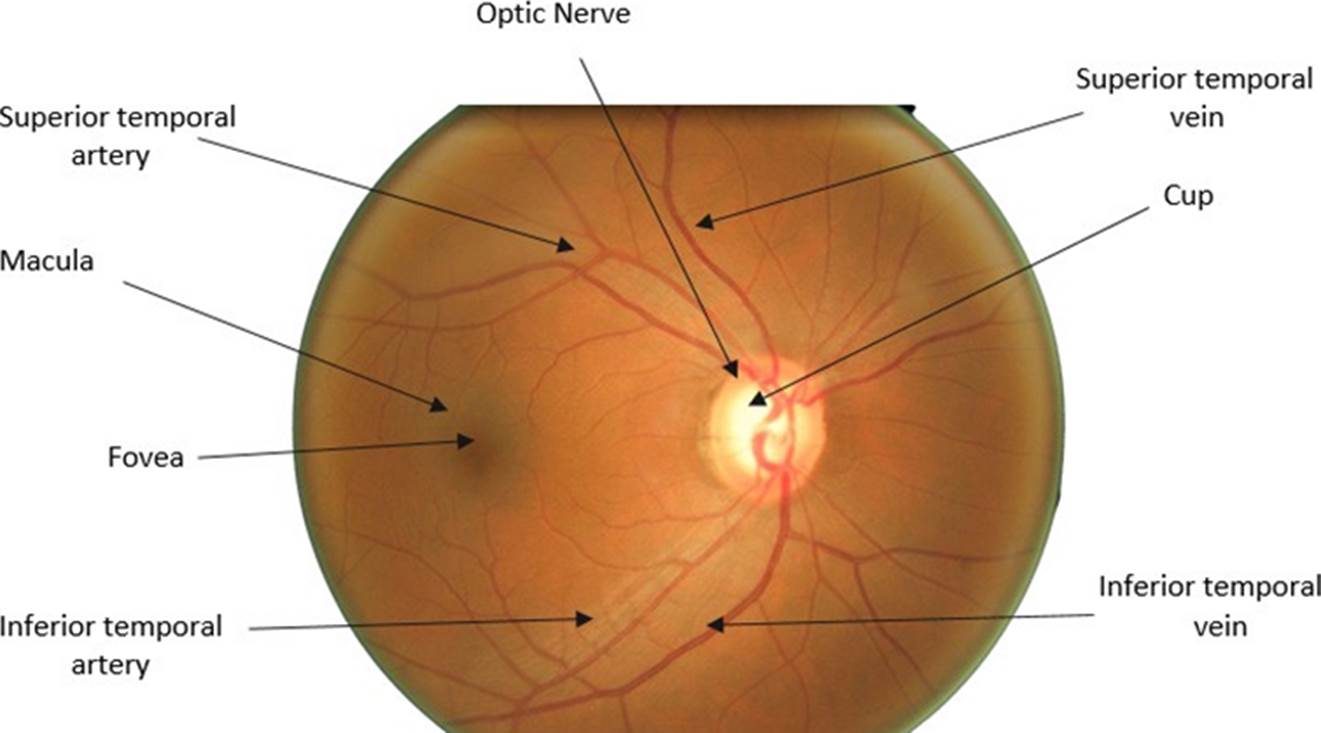
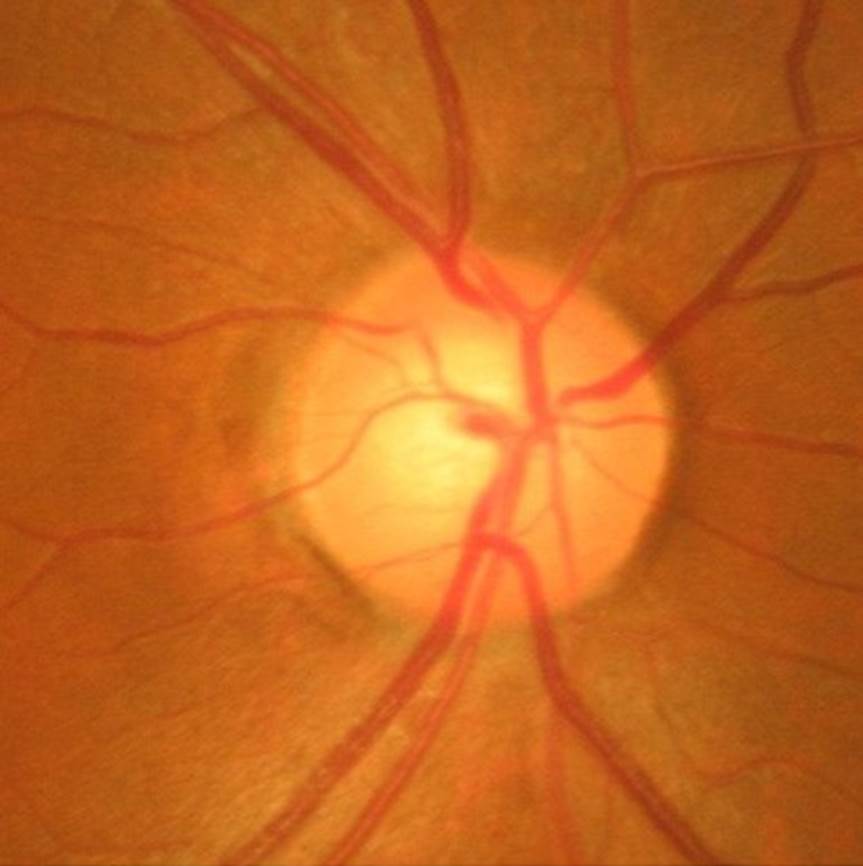
Figure 1 shows an image of the fundus in a healthy condition where the most important parts can be seen, such as the optic nerve, which is where the study of this work will be focused. The outer part of the optic nerve is called the optic disk (OD), and the smaller blurry inner circle is called the optic cup (OC). In the OD area, we can see the main arteries and veins, whereas the veins have a darker color than the arteries. Veins usually are larger in caliber than arteries, having an average AVR ratio of 2:3 [17].
The region of interest (ROI) usually is less than 11% of the retina's fundus image's total size. By decreasing the size of the image with the ROI's detection, a reduction in the computational resources used is possible [18]. Both optic disc and cup segmentation are essential components of optic nerve segmentation and, together, form the basis of a glaucoma evaluation. In [19], a reference data set for evaluating the cup segmentation method was published. Nevertheless, it does not provide free access to the general public.
There are relatively few public data sets for glaucoma evaluation compared to available data sets for diabetic retinopathy [20] and vascular segmentation [21]. The ORIGA database contains 650 retinal images labeled by retina specialists from the Singapore Eye Research Institute. An extensive collection of image signs usually taken into account for the diagnosis of glaucoma are annotated. In the Drishti-GS dataset [22], all images were collected from the Madurai Aravind Eye Hospital of the hospital visitors with their consent. The selection of glaucoma patients is made based on the clinical findings during the study. The selected subjects are between 40 and 80 years old, and the number of males and females is roughly equal. Patients who choose to undergo routine optometry and who are not glaucoma represent the normal category.
Usually, the fundus image analysis with artificial intelligence is carried out from two approaches, 1) the classification at the image level and 2) the classification at the pixel level. In image-level classification, the learning model is trained with images previously classified by an expert, in this case, a retina specialist. This classification generally contains the disease progression [23]. For example, the severity of DR is classified into five grades, and each of these grades is associated with a number. The learning model begins to associate the patterns in the image to their labels. The second approach is the anatomical and lesion segmentation, such as separating the blood vessels from the rest of the retina in order to measure their caliber. For example, in the case of Hypertensive Retinopathy, the vein/artery relationship plays an essential role in the diagnosis of the disease [24].
There are several works carried out for the detection of glaucoma. Both images based and pixel-based classification have been used. We will follow an imagebased classification approach in this research.
A six-layer CNN architecture was proposed by Chen et al. [5], where four layers are convolutional, and the final two are fully connected. ORIGA and SCES are used in this study. From the ORIGA database, 99 images were randomly selected for training and the remaining 551 images for the testing, obtaining results of 0.831 for AUC. In a second experiment, 650 images from the ORIGA database are used for training, and 1676 images from the SCES database for the testing, the area under the curve obtained is 0.887.
Acharya et al. [6] proposed to use a Support Vector Machine for classification and the Gabor transform that will notice the subtle changes in the image's background. The database used was a private database of Kasturba Medical College, Manipal, India, with 510 images. 90% of the images were used for training, while the remaining 10% for testing. The results obtained were 93.10% accuracy, 89.75% sensitivity, and a specificity of 96.20%.
Raghavendra et al. [1] proposes to perform the automatic recognition of glaucoma utilizing a convolutional neural network of 18 layers. This work consists of a standard CNN, with convolution layers and max-pooling, and a fully connected layer where classification is performed. Initially, 70% of the randomly selected samples are used for training and 30% for testing. 589 healthy images and 837 with glaucoma of a private database were deployed. The process was repeated fifty times with random training and test partitions. The results obtained were 98.13% accuracy, 98% sensitivity, and 98.3% specificity.
Gour et al. [8] proposes an automatic glaucoma detection system using Support Vector Machine (SVM) for classification. Combine GIST and PHOG to extract features in images. This technique eliminates the need for image segmentation. Instead, it works with a diagnostic system that makes use of characteristics such as texture and shape to detect the disease. This technique yielded an accuracy of 83.4% using the Drishti-GS1 and High-Resolution Fundus (HRF) databases.
Gheisari et al. [25] implement two architectures, the VGG16 and ResNet, concatenating LSTM blocks. To determine the best one, they carry out several experiments varying the number of epochs and learning rate. The best results are achieved with the VGG16 network, achieving 95% sensitivity and 96% specificity.
Gómez-Valverde et al. [26] use architectures such as VGG19, ResNet, GoogleNet and Denet Disc. The best results obtained were obtained using VGG19 with transfer learning, obtaining 94.20 of AUC, 87.01 of sensitivity, and 89.01 of specificity.
Pinto et al. [27] use 5 databases adding a total of 1707 images. They carry out the experimentation with each of the databases separately, but the best results were obtained by putting together all the available images. They achieve an AUC of 96.05, a specificity of 85.8 and a sensitivity of 93.46 using Xception architecture.
We propose an image-based classification approach using a deep neural network for glaucoma diagnosis in fundus images in the present work. A preprocessing step will be carried out where the region of interest will be extracted, specifically the region where the optic disc is located. Once that region is obtained, a neural network is fed with the cropped images in order to classify if the image has or not glaucoma.
MATERIALS AND METHODS
Preprocessing
This section introduces a method to locate the retina optic disc, which contains the necessary features to diagnose glaucoma. These image areas will be the in- put to the neural network proposed in this work. Since the images' size is 3072 x 2048 pixels, it is reduced to four times its original size, leaving the images' dimensions in 768 x 512. The input images are converted to grayscale. Therefore, it is reasonable to obtain a higher contrast of the optic disc than the original image. For this, the red and green channels are used, which are the ones that have the most significant impact on the optic disc. To do this, Equation 1 is applied.
Where Imggray is the grayscale image, and R and G are the corresponding red and green channels. To determine which channels would be used, the histograms per channel of the image were obtained, in which it is determined which of them have the greatest impact on the contrast of the image. Conventional grayscale conversion is obtained using the luminance coefficients in ITU-R BT. 601-7, which is a recommendation that specifies digital video signal encoding methods [28].
The coefficients and channels used in our method were obtained by analyzing the histograms in each channel of the images. These histograms are shown in Figure 2.
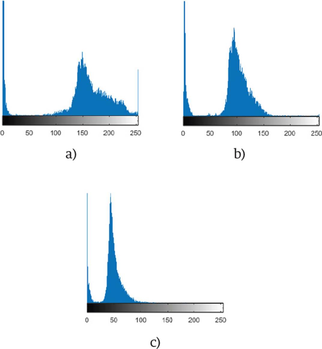
Figure 2 The histogram of the red channel is shown in a), the green channel in b), and the blue channel in c).
The results obtained after the transformation are shown in Figure 3.
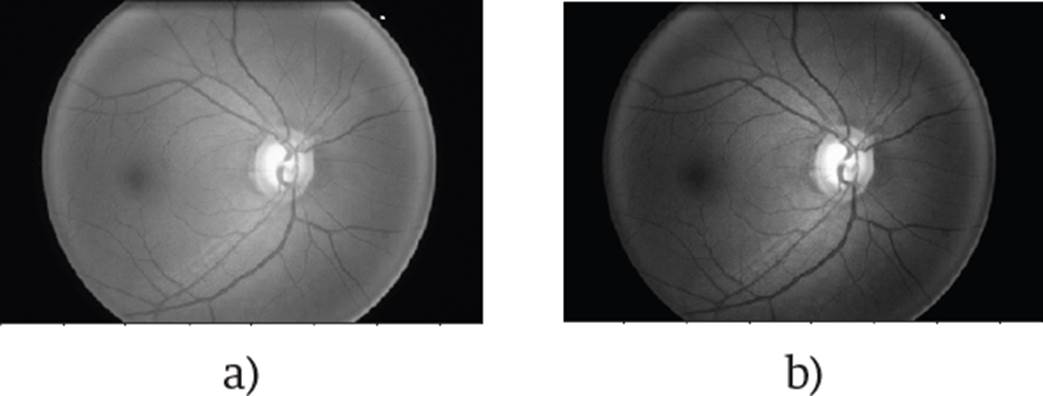
Figure 3 The conventional transformation to grayscale is represented by a), and the one proposed by b).
The next step is to scroll a kernel through the image to divide it into different sub-images to determine where the optic disc is located as shown in Figure 4. The optic disc is the most brilliant part of the retina. Excess brightness can be eliminated in parts where the optic disc is not located.

Because the optical disk represents approximately 10% of the original image, the scrolling box's size, or kernel, was chosen to ensure that any sub-images would be selected. The selected size was 192 x 192 pixels, four times smaller than the image width after size reduction.
Equation 2 is applied to calculate the sub-images, depending on the size of the scrolling box and the step used
Where SubImg is the image inside the kernel, Img is the image after resizing, x is the kernel's horizontal starting point, y the vertical starting point, x0 the horizontal endpoint, that is, x + 192 and y0 the vertical endpoint, that is, y + 192.
To reduce the processing time, the kernel step will be 165 pixels in the horizontal direction and 150 in the vertical direction. With this step, we guarantee that the optical disc is in one of the sub-images at least once. Each time a new sub-image is selected, the average of all the pixels is calculated by applying Equation 3. This average is stored, and once all the sub-images have been analyzed, it is located where the highest average is. In this way, the sub-image where the optic disk is predicted is chosen.
Where promPix is the average of the pixel values, pi is the current pixel value, and n is the total number of pixels. With this new sub-image selected, the pixels' average value is taken, but now of each column and row.
This average will give us x and y coordinates. These coordinates represent the new image center that will be cropped to obtain the ROI. An example of this can be found in Figure 5.
The result after cropping an image can be found in Figure 6.
The entire process explained above for the ROI detection is shown in the pseudo-code in Algorithm 1.

The preprocessing described in Algorithm 1 is applied to the 650 images of the ORIGA database [16] to obtain the ROI. With the region of interest located, we proceed to perform normalization to the images. What is sought is that the values are within a smaller range, since the CNN’s do not perform well when the input numerical attributes have a very large range. The normalization used (Equation 4 was the min-max [23].
Where valNorm is the normalized value, val is the current value, minimg and maximg are the minimum and maximum image values. The values before normalization range from 0 to 255. After normalization, they will be in a range from 0 to 1.
Architecture
The images fed to the network have a size of 128 x 128 pixels. Convolution layers, ReLU, max-pooling, and fully connected layers comprise the proposed neural network. The output of each layer is the input of another, thus allowing the extraction of features. Since it is sought to differentiate between small and local image characteristics, which may differentiate a person's distinctive features with glaucoma, small 3x3 and 5x5 filters are used in the network. The final two layers will unite these characteristics to make a classification.
The order of the layers; convolution, ReLu and max-pooling is used in several well-known architectures, such as VGG16 [29]. The idea of using two fully connected layers came from the AlexNet [30] network, which uses 3 fully connected layers. Based on these two articles, an architecture is proposed.
As activation function at the output of the network, the sigmoidal function was used. This function was chosen because we are interested in a binary classification, so it will give us a probability of which class it can belong to. This activation function should not be confused with the one used between each convolutional layer. ReLU is used to add non-linearity to the network and sigmoidal is used to regularize the output. The first fully connected layer has 128 neurons and the second has 2 neurons for classification.
As a loss function, we use Binary Cross Entropy. This was chosen due to the fact that binary classification is sought. This function will give us the prediction error, which will indicate to the network how correct its classification, which will help the network to improve as they pass the epochs. To avoid overfitting, dropout was used, which randomly turns off neurons in each training period, in order to distribute the power of selection of characteristics to all neurons equally, in this way, the model to learn independent characteristics. Adam was used as an optimizer, which combines the advantages of some others, such as the Momentum, maintaining the exponential moving average of the gradients, and the RMSprop, which maintains the exponential moving average, but of squared gradients.
The proposed neural network consists of fifteen layers. This number of layers was determined by experimentation. We have to take into account that with a shallower network, the extraction of features could be poor and therefore increase the difficulty to identify the desired features. However, with a deeper architecture, there is a risk of overfitting.
Convolutional layers represent high-level data features, and combining with a fully connected layer is one way to learn non-linear combinations of those features. In the network, two completely connected layers are used, seeking more significant learning of these combinations. To choose the best learning rate, we carried out tests with different values, and the one that had a better relationship between learning rate and performance is the selected one. The two images where the optic disc was not correctly detected are shown in Figure 8.
In images that were not appropriately cropped, excess brightness may be noticed on the circumference of the fundus image. For this reason, the algorithm places the optic disc in that position and does not cut the image correctly. Of the 650 used images, 482 are from healthy patients and 168 from glaucoma patients.
Training and testing
455 images were used for training and 195 for validation, that is, 70% for training and 30% for validation. The images were chosen at random. The algorithm was developed in Python and ran on a computer with an Intel Core i7-3160QM 2.3 GHz CPU and 8 GB of RAM. The training execution time was 18.5 hours. Python 3 and TensorFlow were used. To implement the algorithm, it was necessary to use the Keras, Pandas, Numpy and Matplotlib libraries.
To ensure the obtained results were correct, we implemented cross-validation. For this validation, the algorithm was executed ten times for a k-fold with a value of k = 10. Each of the executions had 50 epochs. The advantage that it gives our model the opportunity to perform multiple training-test partitions. This can better show how our model performs on unseen data.
RESULTS AND DISCUSSION
For evaluation of the obtained results, some metrics such as accuracy, sensitivity, and area under the curve were used:
True-Positives (TP): The predicted value was positive and agreed with the true value.
True-Negatives (TN): The predicted value was negative and agrees with the true value.
False-Positives (FP): The model is classified as a positive class, and the true value is negative.
False-Negatives (FN): The model is classified as a negative class, and the actual value is positive.
Accuracy tells us the percentage of predictions that were made correctly.
The sensitivity tells us how many of the positive cases the model was able to predict correctly.
The ROC-AUC is the metric that shows us a probability curve, which is shown by sketching the range of true positives against the range of false positives at various threshold values. The results obtained with different learning rates without ROI are shown in Table 1.
Table 1 Performance without ROI.
| Learning rate | Accuracy | Sensitivity | ROC-AUC |
|---|---|---|---|
| 0.01 | 88.72 | 89.42 | 89.71 |
| 0.001 | 90.01 | 90.01 | 90.35 |
| 0.0001 | 91.02 | 93.01 | 89.14 |
The results obtained with different learning rates and ROI are shown in Table 2.
Table 2 Performance with ROI.
| Learning rate | Accuracy | Sensitivity | ROC-AUC |
|---|---|---|---|
| 0.01 | 91.36 | 92.62 | 92.87 |
| 0.001 | 92.13 | 93.18 | 92.57 |
| 0.0001 | 93.03 | 94.02 | 93.56 |
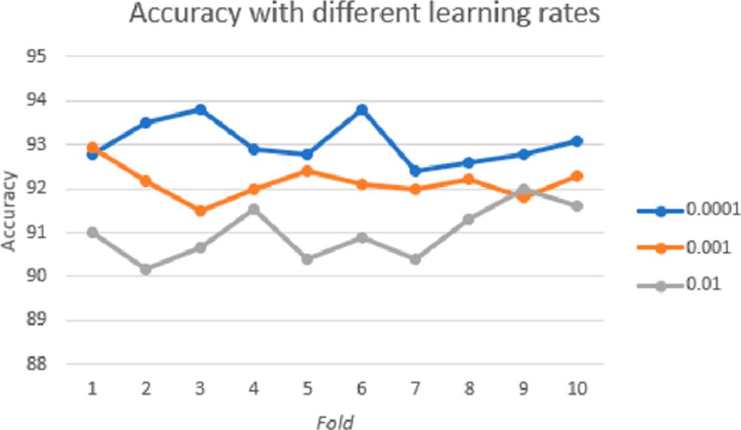
Figure 10 shows the graph obtained for ROC-AUC, threshold values are in intervals of 0.01.
In order to check on which part of the image the network was more focused to perform the classification, it was decided to obtain a method of visualization of neuron activations. There are several options to perform this task. Erhan et al. [31] propose a method that seeks to produce an image that shows the activation of the specific neuron we are trying to visualize. Zeiler et al. [32] propose a method to find the patterns of the input image that activate a specific neuron in a layer of a CNN. Dosovitskiy et al. [33] propose a method that consists of training a neural network that performs the steps in the opposite direction to the original one so that the output of this new network is the reconstructed image.
The method used in this work is the one proposed by Selvaraju et al. [34] that adopts a CAM architecture, which generates a class activation map that indicates the most used image regions. Retraining is required for this purpose. In Figure 11 we can visualize the regions in the image that have the most weight while making the classification in some of the images.
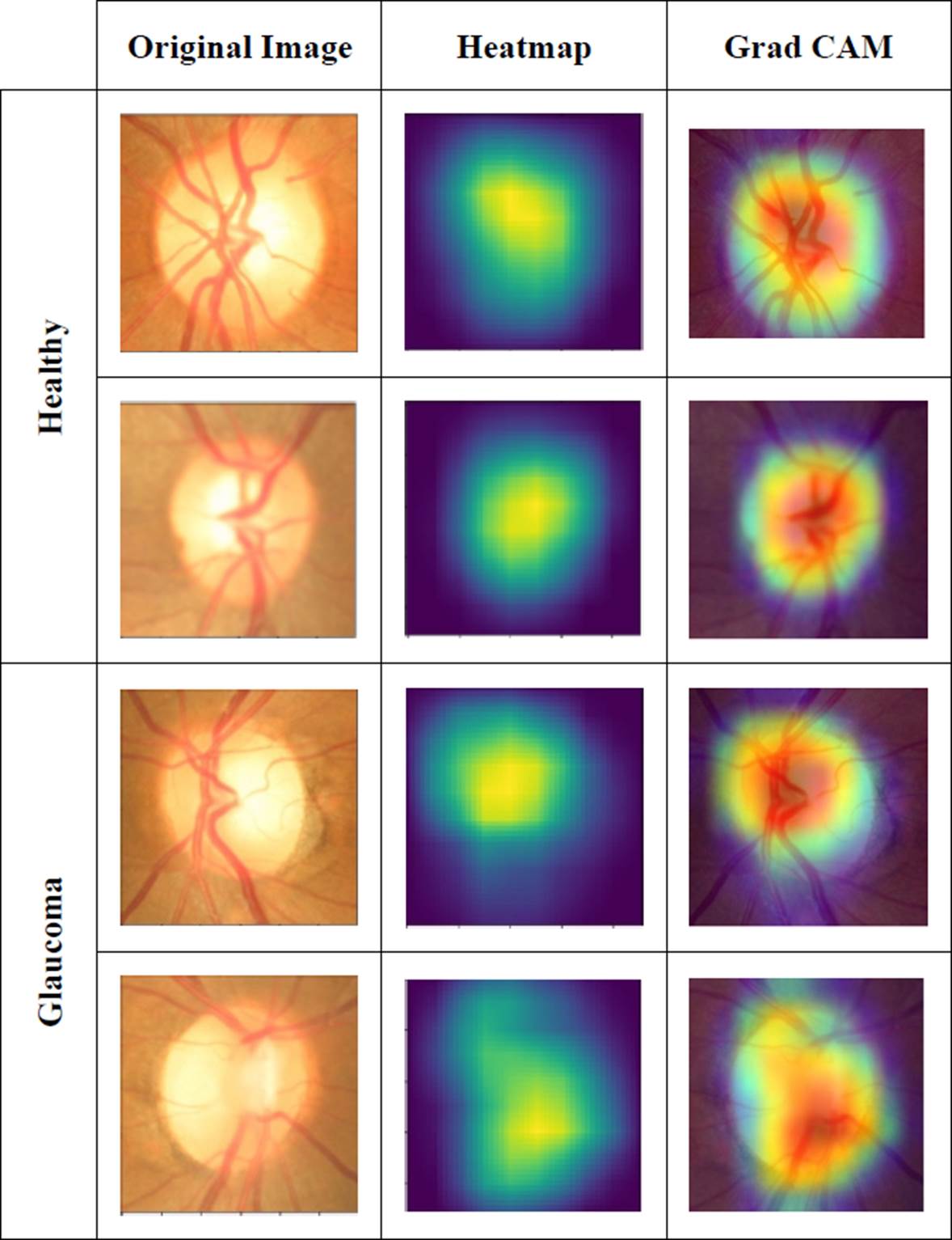
For the color map, the Jet configuration was used, which returns a color map in a three-column matrix, with the same number of rows as the color map of the original image.
Each row will have different intensities between the color red, green, and blue.
Table 3 compares the performance of our method against other methods found in the literature. It outperforms all other results in any of the displayed metrics.
Table 3 Comparison of our method against other methods of state-of-the-art.
| Method | Performance |
|---|---|
| Six layers CNN [5] |
ROC-AUC: 88.7 |
| Different features from Gabor transform (SVM) [6] |
Accuracy: 93.1 Sensitivity: 89.75 Specificity: 96.2 |
| Eighteen layers CNN [1] |
Accuracy: 98.13 Sensitivity: 98 Specificity: 98.3 |
| GIST y PHOG (SVM) [8] |
Accuracy: 83.4 ROC-AUC: 88 |
| VGG16 + LSTM [25] |
Sensitivity: 95 Specificity. 96 |
| VGG19 + Transfer learning [26] |
ROC-AUC: 94.2 Sensitivity: 87 Specificity: 89.01 |
| Xception [27] |
ROC-AUC: 96.05 Specificity: 85.8 Sensitivity: 93.46 |
| Proposed |
Accuracy: 93.03 Sensitivity: 94.02 ROC-AUC: 93.56 |
CONCLUSIONS
As we stated, glaucoma is one of the principal causes of blindness globally. It could be vitally important to have a tool capable of supporting ophthalmologists to diagnose this condition more quickly.
The proposed method achieves excellent metrics with a not-so-deep neural network, achieving an accuracy, sensitivity, and area under the curve of 93.22, 94.14, and 93.98, respectively. To corroborate the performance of our approach, we did our analysis on the ORIGA database, which is public, and it is one of the most used databases for glaucoma analysis.
The preprocessing of the images to obtain the ROI also helps the algorithm be more effective. It obtains the region where the optical disc is located in almost all the images of the database used, being a method to use in future work.
We will further examine different alternatives to increase the classification performance, either by preprocessing or modifying the network structure.
The purpose of this investigation is to get a high classification method that could be implemented for automatic glaucoma detection; this would save specialists time and speed up the diagnostic process.
By obtaining the characteristics map, we were able to visualize in which part of the image the decision of the network has more weight. Therefore, we conclude that the decision is made depending on the disc and optical cup characteristics, as shown in the results.
For any reader that would like to see the implementation code, it can be provided by requesting it to the corresponding author.

