


 nueva página del texto (beta)
 Inglés (pdf)
 Artículo en XML
 Referencias del artículo
 Enviar artículo por email
 Citado por SciELO
  Similares en
SciELO
Similares en
SciELO 
 Permalink
Introduction
In areas of scientific research where imaging is involved (e.g., neuroimaging, remote sensing, etc.), it is often necessary to test statistical hypotheses at each element of a 2 or 3-dimensional field of sites (pixels or voxels). The purpose is to determine the set of sites at which the response to a given experiment may be different from baseline, or whether it is significantly correlated with another parameter.
For instance, researchers in the area of neuroscience typically conduct studies to identify the area of the brain responsible for a certain cognitive task. The experiments are composed of stimulus and rest periods applied to a single subject or several people[1,2,3,4,5], applying a functional imaging approach such as positron emission tomography (PET) or functional magnetic resonance imaging (fMRI). Subsequently, the regions of voxels with a significant degree of activation have to be detected by performing simultaneous hypothesis tests over 2 or 3-dimensional measurements.
Because hundreds of thousands of comparisons are made at the same time, the well-known problem of multiple comparisons appears[6,7]. The researcher is thus obliged to seek a solution to the resulting increase in the percentage of false positives (type I errors). A popular family of approaches to deal with this problem are the so-called pointwise (PW) methods, which utilize some type of thresholding technique to control the family-wise error rate (FWER)[6,8]. Although they present a simple and easy to interpret solution, there is a high rate of type I errors.
Some authors address the problem through the Gaussian random fields (GRF) theory[9,10], under the assumption that the spatial correlation of the data is known or can be estimated. Since this is not true in practice[11], a smoothing filter is applied to the raw images to ensure that these assumptions are met. Such a pre-processing process causes a loss of spatial resolution[5]. On the other hand, threshold-free methodologies[12] employ erosion and dilatation morphological operators with a set of structuring elements of various sizes to detect regions exhibiting moderate activation levels and wide spatial size. However, their results are subject to the form of the structuring elements, which is determined arbitrarily.
In the current contribution, we propose a new method, denominated the regularized hypothesis testing (RHT) method. It is based on the formulation of the hypothesis testing task as a Bayesian estimation problem using a Markovian random field (MRF) to incorporate local spatial information. Firstly, mention is made of the state-of-the-art methods available to solve the problem of hypothesis testing in 2 and 3-dimensional fields. Thereafter, RHT is explained along with related theoretical considerations. The problem of parameter selection is addressed by proposing two algorithms for automatic calibration. Having laid out the new method, it is validated by experiments with simulated and real data. Finally, the results are discussed and conclusions are drawn.
Theoretical framework
The problem of testing statistical hypotheses at each element of a 2 or 3-dimensional field can be conceived as the following general problem:
Given a set
where H0u is a marginal null hypothesis about
the probability distribution of the measurements at site u. At
H0u, consequently
Once a method is selected, its performance must be evaluated with standard tools. Some very common tools that will be used presently are described.
where
It is also possible to define FPR for elements that are not adjacent to the boundary of the active region:
where the r-dilation
This measure is defined for two reasons. Firstly, the boundary of the active region is
usually not well localized, since the activation level often decreases slowly as
one moves away from
Thus,
denoting the expected proportion of sites correctly estimated as the activation region.
representing the probability Pr of having at least one false positive, given that the activation region is empty.
with
portraying the proportion of wrongly rejected null hypotheses in
Some of these measures can be combined. For example, a widely accepted way of characterizing the performance of a method is through the receiver operating characteristic (ROC) curve[13], which indicates, for a fixed
To construct the curve, the true region
where pv(u) depicts the p-value of
where
In the case of FDR, with a significance level
αFDR[16], the procedure for finding the threshold
θ begins with ordering the individual p-values of sites
and θ is set as:
For more details on the method, consult Benjamini [17]. Alternatively, given a desired value ϵ for FPRmax, θ can simply be set as ϵ (e.g., ϵ= 10-5). If the local hypotheses H0u are independent, this is equivalent to the application of the standard PW method without correction for multiple hypotheses, but with low level of significance α = ϵ. Since (as mentioned) the maximum TPR is an increasing function of FPR, the value of θ* = ϵ will be the one that maximizes the TPR while keeping FPR under control:
where ϵ is a user-specified small positive number. Although the actual ROC curve for a given problem is unknown (because it depends on the values of
The signal-to-noise ratio (SNR) [20] is defined as:
where σ0 is the variance of
Consequently, PW methods have low sensitivity and the estimated
Hence, more sensitive methods must be developed that are able to accurately reflect the active regions, which in most cases consist of clusters of several contiguous elements of
However, this approach has some drawbacks, one being that the results depend strongly on the value of the selected threshold, and in general no principled way exists to make such a selection. Some variants of the method alleviate the problem to a certain extent by computing
A distinct approach was developed to address these problems, being the morphology-based hypothesis testing (MBHT) method[12]. It involves the computation of
where Wk(u) denotes the structuring element
k (e.g., a circle of radius
rk) centered at
u. Then, these values are integrated into the statistic
where P0K is the null distribution of the
statistic
The results of this approach are competitive with those based on supra-threshold cluster statistics[12] and allow a clearer interpretation. Once again, the disadvantage is that the results may depend on the shape of the structuring elements, and for their selection no principled solution exists.
In the current contribution, the approach introduced is capable of overcoming these difficulties. It formulates the hypothesis testing task as a Bayesian estimation problem, with an MRF previously applied to the active regions, thus implementing a prior constraint on the spatial contiguity of
The new scheme proved to have better performance than PW methods, while maintaining interpretability. It also has better performance than MBHT, and does not require the selection of any particular shape for the structuring elements.
The regularized hypothesis testing method
In RHT, the hypothesis testing problem is written in terms of an image segmentation problem, which is solved by using a Bayesian estimation framework. First, the hypothesis testing formulation is explained. The procedure is laid out for calculating the prior distributions of sites and the likelihood that they belong to an active region. Subsequently, an approximation algorithm for finding the maximum a posterior probability (MAP) estimate is established. Finally, the parameter selection problem is addressed.
Hypothesis testing formulation
Hypothesis testing may be formulated as a binary segmentation problem. Accordingly, given the
set of sites
Let
c
be an unknown discrete label field that identifies the partitions of
Without loss of generality, the activation level in
where n is a noise field showing distribution Pn(n), with:
where Zn is a normalization constant and
Un(n) is a
so-called energy function. Then, the likelihood
where
As the real statistic
Noise field model
For the noise field n, a GMRF model was employed, taking the form of Eq. (16) with:
where γ > 0 is a scale parameter, n(u) is
the value of the field n in site u, and
n(v) is the value of the field
When τ1 = 0 and γ = 1, the formulation is reduced to a Gaussian white noise model with zero mean and unit variance (the “Parameter Selection” section explains other types of noise fields). With such a model, the likelihood takes the form of Eq. (17), being:
In the above equation, c(u) is used as an
indicator function. Accordingly, if its value is 1 (i.e., u ∈
Moreover, if
c(u)=0 (i.e.,
Eq. (19) may be rewritten as a quadratic function of a vector-valued field b defined as b1(u) = c(u) and b0(u) = 1 - c(u),
with
Bayesian formulation of the hypothesis testing problem
For field b, we propose the previous application of an MRF model [22,23]. In order to introduce the prior constraint that the active regions are spatially cohesive, b is modeled with Ising potentials, furnishing the following distribution:
where τ2 ≥ 0 is a parameter that controls the granularity of field b.
With this equation and the Gauss-Markov model (16) and (18) for noise, it is possible to estimate field b by employing a Bayesian formulation, affording the posterior probability distribution:
where the likelihood is:
with
where
The MAP estimate for field b is obtained by minimizing (28), subject to the constraints (21)-(22). This is a combinatorial optimization problem that is, in general, very difficult to solve. Several methods have been proposed, such as the iterated conditional modes (ICM) algorithm[24], stochastic relaxation[25], graph cuts procedure[26], etc.
Here, because of the form of the cost function that includes the noise correlation term, we prefer option[22], which is based on the relaxation of constraint (22). Hence, a new formulation is made:
Dividing (28) by γ and utilizing
If the noise has a mean of zero, then α0 = 0. The resulting optimization problem is:
This is a quadratic minimization problem, subject to linear constraints, which can be solved
efficiently by employing a projected gradient descent method. Consequently, each
b(u) (in order to simplify the notation we
remove the dependency of ν, α1,
λ) may now be interpreted as an approximation for the
posterior marginal distribution of the indicator functions
To obtain the latter it is possible to set
Parameter selection
A general method can now be introduced to allow the model (31)-(33) to be used for any type of noise. The parameters α1, ν, λ will be able to be automatically selected by controlling the false positive proportion while maximizing the performance of the method with respect to the TPR.
Standardization of the noise field
The derivation of functional (31) is based on the observation model (15) with the Gauss-Markov model (16)-(18) for noise. However, the model is not always valid in practice, since the
If
If u is a uniform random variable and G the CDF of the normal distribution, then the distribution function for the random variable G -1 (u) is normal [29].
Combining both properties, it follows that for any random variable x, the random variable G
-1 (Q(x)) is normal. Consequently, the only requirement for transforming a random variable x into a normal variable is to know the corresponding CDF Q(x) or to estimate it by obtaining the empirical CDF (ECDF)
Assuming that random field samples
where erf(y) denotes the error function[30], the probability that a random variable Z normally distributed with mean μ = 0 and variance σ = 1/2 falls in the range [-y,y]. The field
Hyper-parameter calibration
The hyper-parameters that control the behavior of the method are the spatial correlation parameter ν, the minimum activation level α1, and the regularization parameter λ. The general idea is to estimate ν from the observations, and subsequently compute α1, λ from the estimated parameter ν and a parameter ϵ representing the level of FPR control.
Estimation of parameter ν: The parameter ν =
τ
1/γ in (31) controls the noise spatial correlation and can be estimated by
minimizing the negative logarithm of the pseudo-likelihood of samples of the
field
The pseudo-likelihood is defined as the product of the conditional distributions for n(u) at each pixel u, given the values at its neighboring fields [31]. Using Eqs. (17)-(18), the result is:
where t is a constant,
The minimization of Eq. (37) yields a closed formula for the estimation of the parameters:
Calibration of parameters α1,
λ: For a given value ϵ for FPR control and a
fixed
1. Instead of FPR ≤ ϵ, we use FPR2 ≤ ϵ, Eq. (3), since the precise location of the boundary of the active region
2. According to our experimental work (see Figure 2 and Experiment 1 below), the present method has the advantage that false positives do not extend, in a significant way, more than a couple of pixels away from this boundary. This is due to boundary effects close to the active region. For a given fixed α1 and λ, therefore, it is possible to estimate the constraint FPR2 ≤ ϵ by FPR0 (i.e., the FPR computed in fields generated under H0), which is depicted by FPR0(α1, λ).
3. The calculation can be further simplified based on the observation that TPR is an increasing function of FPR (i.e., the usual shape of the ROC curves). Consequently, for a fixed λ:
which is equivalent to finding α1(λ), such that FPR0(α1(λ), λ) = ϵ. Given that
4. Since the TPR depends on the unknown
where P(α) is taken as the uniform distribution in the set
S. With these simplifications, the parameter estimation
algorithm simply consists of sweeping the plausible λ values in
a given set Λ (a discretization of an interval [0,
λmax]), followed by finding, for each
λ, the value
Algorithm 1: Calibration parameter algorithm (CPA)
| 1 | function CPA(ν, ϵ) | |
| Input | Estimated value of ν from (44); desired control ϵ for the FPR; search interval Λ for λ. | |
| Output | Estimated hyperparameter values a1*, λ* | |
| 2 | Begin | |
| 3 | For all λ ∈ Λ do | |
| 4 | Compute |
|
| 5 | Compute |
|
| 6 | End | |
| 7 | Compute |
|
| 8 | Compute |
|
| 9 | Return a 1*, λ* | |
| 10 | End | |
The optimal parameters α1*, λ* depend on the data only through the estimated parameter ν and the desired FPR0 control ϵ. Thus, the optimal values may be pre-computed and stored in a table. When a new data set arrives, one only needs to standardize the noise, estimate ν, read α1*, λ* from the table for the desired FPR control, and minimize U (b; ν, α1*, λ*) furnished by Eq. (30). The tables are represented as false color images in Figure 1.
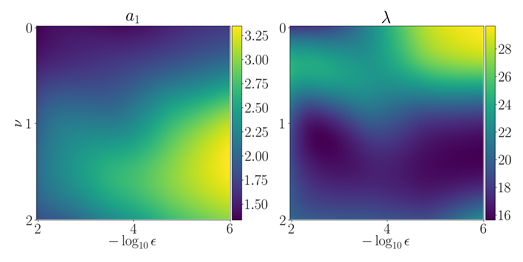
Figure 1 Estimation of parameters a 1, λ as functions depending on (ν, -log10 ϵ) for ν ∈ [0, 2] and ϵ ∈ [106, 10-2].
The final algorithm for estimating the active region
Algorithm 2: Regularized hypothesis testing (RHT) algorithm
| 1 | function RHT |
|
| Input | Observed field |
|
| Output | Estimated active region |
|
| 2 | Begin | |
| 3 | Compute |
|
| 4 | Compute |
|
| 5 | Compute |
|
| 6 | Compute |
|
| 7 | Compute |
|
| 8 | Compute |
|
| 9 |
Return |
|
| 10 | End | |
Materials and methods
Data description
To study the behavior of the present method, we include various experiments based on both synthetic and real data.
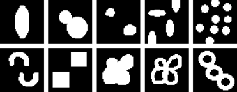
Synthetic data: The synthetic data was generated dynamically and consisted of
two components. Firstly, S0 =
{n1, n2, …,
n40} is a set of noise fields of a regular
lattice
where α denotes the activation level and its value is specified in each experiment.
Real data: Experiments with real data were based on the auditory dataset[32]. The data corresponded to 96 volumes of a single subject (each volume composed of 64×64×64 voxels of 1×1×3 mm), which were acquired in blocks of 6 volumes. Since the repetition time between scanning was set to 7 seconds, there were a total of 16 blocks of 42 seconds (although due to the effects related to T1, the first two blocks were discarded). The sequence of volumes alternated between blocks of rest and stimulation, starting with rest. Auditory stimulation consisted of two-syllable words presented binaurally at a rate of 60 per minute.
Localization of false positives for the RHT algorithm
This experiment was designed to test the assumption that in the proposed method the false positive errors are concentrated close to the boundary of the active region. Consequently, FPR2 can be well approximated by FPR0 (i.e., FPR computed over images produced under H0).
A total of 1000 independent runs were conducted for the procedure. Briefly, set S0 was generated with parameter ν = 0.75, a value estimated from fMRI images by utilizing Eq. (44). Fields T1, T2, …, T40 were obtained by using model (47), sets S0 and S1, and randomly selected activation level α in the interval [2,4].
Algorithm 2 was applied for levels of FPR control ϵ ∈ {0.001, 0.0001, 0.00001, 0.000001} with the optimally calibrated parameters, computing the average value of FPR2 for the set S1and FPR for the set S0. The results are shown in Table 1. As can be appreciated, by calibrating the parameters of the method to control FPR0, the appropriate control over FPR2 is also achieved.
Table 1 Experiment of the FPR control at different levels, utilizing a synthetic dataset. First column, level of FPR control; second column, average FPR for images generated under H 0; third column, average FPR 2 for synthetic active regions.
| ϵ | FPR0 | FPR2 |
|---|---|---|
| 0.01 | 0.0042504 | 0.0051335 |
| 0.001 | 0.0001340 | 0.0001714 |
| 0.0001 | 0.0000436 | 0.0000436 |
| 0.00001 | 0.0000044 | 0.0000050 |
| 0.000001 | 0.0000004 | 0.0000004 |
Performance of the method
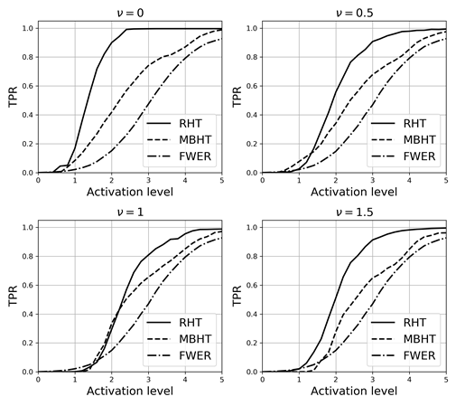
The first set of the following experiments was designed to make a comparison of RHT to FWER [8] and MBHT [12], the latter two being the state-of-the-art methods that take the spatial expanse of the active region into account. Accordingly, the set S
0 was produced with parameter ν ∈ {0, 0.5, 1, 1.5}. A total of 1000 runs were performed, randomly selecting the active regions
Based on the results from each method, RHT proved capable of providing better TPR values than the other two algorithms for most activation levels (Figure 3). The improvement is likely due to the consideration in the new model of the spatial cohesion of the activation regions (controlled by the regularization parameter λ) as well as the spatial correlation in the noise field (controlled by the parameter ν). Contrarily, the rest of the algorithms assume that these two components of statistic T are formed by independent variables.
Experiments with fMRI data
In the second set of experiments, Algorithm 2 of the proposed method was applied to the real fMRI data described at the beginning of this section. RHT was not applied directly to the original data, but rather to a field T (an F-test field computed from the data). The first step was to standardize the field in order to obtain
Data pre-processing. The aim of the pre-processing was to remove artifacts in the data as well as to prepare the data to maximize the statistical analysis. Here we use spatial pre-processing provided in the script auditory_spm12_batch.m, which implies realignment, co-registration, segmentation and normalization. Although the original script (available online at http://www.fil.ion.ucl.ac.uk/spm/data/auditory/) includes a smoothing step to ensure that some assumptions about noise distribution are fulfilled[11,18], RHT omits this step because it is capable of handling different noise distributions. Actually, the inclusion of the step would not be beneficial. The data for these calculations was processed on SPM software version 12 (available at http://www.fil.ion.ucl.ac.uk/spm/) and MATLAB 2018a. A slice of the pre-processed data was selected to perform the following experiments.
F-test field. After the pre-processing stage, the statistical analysis was carried out to determine the active voxels that correspond to a given stimulus. To obtain the active regions, a voxel-wise analysis is typically conducted by fitting models to a single voxel time course. The data at each voxel is modeled in a univariate way with a linear model:
where yt, the dependent variable, is a vector formed by the intensity values at each time point. β0 and β1 are the intercept and the slope of the linear model, respectively. Meanwhile, ϵt is the error term in the model fitting, which captures factors other than xt, such as signal noise, capable of affecting yt. The explanatory variable xt corresponds to the model of neural activity. It is also a vector comprised of entries depicting a real value at each time point:
where ht stands for the hemodynamic response function and dt ∈ {0,1} is an impulse train that indicates whether the stimulus was present at time t. Then, the neural activity is modeled as a convolution,* in which the hemodynamic response function acts as a filter.
The F-test represents the ratio between the variance described in a reduced model yt = β0 + ϵt (without any additional effect) and the full model (48)-(49) that includes the effect of interest. Finally, the F-test was computed for every voxel in the volume. The resulting field was the input for the RHT algorithm, calculated by using the script auditory_spm12_batch.m with the default parameters.
Null distribution. Before the segmentation step of the RHT algorithm, it was
necessary to normalize the F-test field and thus to estimate
the null distribution. More specifically, a sample of the
F-test was obtained under H0,
allowing for the computation of the corresponding ECDF. This was carried out by
permuting the order of the stimulus labels
d(t) for the volumes (see [33] for more details), and by calculating
the F-test field for each permutation, as explained in the
previous section. After completion of these procedures, it was possible to apply
Eq. (36) to transform the
original F-test field (i.e., the original order of the labels
d(t), without permutation) to one that
follows a standard normal distribution. Finally,
RHT algorithm robustness with respect to SNR
In order to investigate the stability of the present method, the algorithm was tested by modifying the SNR in the data from which the activation region would be established. Accordingly, blocks of observations were eliminated from the full experiment. As aforementioned, the first two of the 16 original blocks were eliminated due to effects related to T1. Hence, 14 blocks (84 volumes) were taken initially to perform the procedure described earlier in this section to identify the activation regions. Subsequently, the number of blocks was reduced by two, taking 12 blocks (72 volumes) and performing the procedure again to determine the activation regions, and so on until reaching 4 blocks.
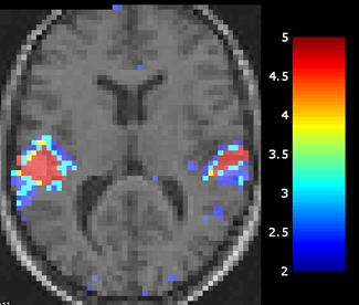
In each case, a tolerance for false positives to ϵ = 0.0001 was established and the results of RHT were compared to those obtained with MBHT and FWER using the same number of blocks. It can be verified by visual inspection (Figure 4) that the three methods− RHT, MBHT and FWER− detected activation regions corresponding to the primary auditory cortex, located at the upper sides of the temporal lobes, specifically on the transverse temporal gyri [34,35].

Figure 4 Performance comparison of the RHT, MBHT and FWER by modifying the SNR in the data through the elimination of blocks.
The MBHT and RHT methods afforded better performance and robustness for the reduction of information in most cases. MBHT and FWER displayed less accuracy when reducing the signal information for ϵ = 0.00001. While FWER exhibited difficulties in the identification of activation regions with 6 and 4 blocks (barely finding any region), RHT and MBHT gave better performance. However, when the number of blocks was decreased to only 4, MBHT was not able to detect any activation region, while RHT still had a proficient outcome. RHT outperformed the other models two by successfully recovering both regions.
Degree of false positive control. To avoid having to specify a particular value
for ϵ, it is possible to estimate
where
Results and discussion
We herein describe a new method, RHT, for detecting active regions in random fields. The focus is on applications for neuroimaging. With the present method, the expected TPR is maximized while the false positives are kept under control by specifying an upper bound ϵ on FPR0 (the FPR under H0). By making ϵ small enough, there is an effective correction for multiple hypotheses since the total number of false positives in the entire field is controlled. We demonstrated experimentally that most of the false positives produced by RHT are confined to the vicinity of the boundary of the active region. Thus, ϵ also bounds the FPR in the data outside of this boundary (i.e., the FPR2).
Conclusions
The main contributions of the present model are the following:
A Bayesian formulation of the hypothesis testing problem in random fields was reduced to an image or volume segmentation problem, for which the maximum a posteriori estimate could be calculated.
A new Markovian random field model for correlated noise was implemented, from which the appropriate prior distribution could be computed.
A method for estimating the hyper-parameters of the model was conceived, involving two main factors: a) the application of a closed formula for the noise correlation parameter ν based on the maximization of the pseudo-likelihood of the data, and b) a pre-calculated lookup table (independent of the data) for the λ and α 1 parameters. This method makes the whole procedure computationally efficient, since the only thing needed for its application is a way of generating sample images from the null distribution. Such samples can be obtained, for example, by using permutation procedures.
To avoid having to specify a particular value for the ϵ parameter, we demonstrated how to present a family of solutions for different values of ϵ in a single image (the DFPC map), similar to the classic p-value maps.
The performance of the method was validated with synthetic and real data (fMRI images). In both cases, RHT provided an improvement in the TPR (while maintaining the FPR under control) compared to the competitive state-of-the-art methods (MBHT and FWER). For the fMRI data, RHT displayed the best sensitivity, which was particularly high for low SNR.
For simplicity, in the current analysis we focused on two-dimensional data. However, it is possible to directly extend the method to 3D simply by considering an extended neighborhood (e.g., 6 or 26 neighbors for each voxel) in the prior MRF models for the active region and the noise, at the expense of an increased computational complexity.
Although the example application here corresponds to fMRI, the RHT method may be applied to any situation involving the testing of a field of local hypotheses, such as the ones that are common in neuroimaging, remote sensing, and so on.

