


 nueva página del texto (beta)
 Inglés (pdf)
 Artículo en XML
 Referencias del artículo
 Enviar artículo por email
 Citado por SciELO
  Similares en
SciELO
Similares en
SciELO 
 Permalink
INTRODUCTION
Quorum Sensing (QS) is a mechanism of bacterial gene regulation used to coordinate collective behaviors in a population [1]. Among the known bacteria that use the QS mechanism, the Vibrio harveyi is one of the most versatile, mainly because uses the Autoinducer-2 (AI-2) as a signaling molecule which is known as an interspecies signaling molecule [2]. Despite many models have been proposed to describe the QS mechanism [3], just a few of these models are focused on QS mechanism that uses AI-2 as a signaling molecule [4],[5].
Mathematical modeling has become an important tool in many sciences, mainly because of its capability to describe different aspect and relations between the elements of a system. Normally, mathematical models contain a set of parameters which either can be inferred from experimental data, or need to be estimated, and before a mathematical model can be considered reliable, the unknown parameters need to be estimated [6].
When experimental data from the real system is available, the model parameters can be estimated by minimizing a cost function which measures the error between the experimental data and model outcome. Nevertheless, because the quality or quantity of experimental data, the model parameters can present estimation problems, like non-identifiability or parameter uncertainty. These problems are very common in mathematical models that describe biological systems, due to their stochastic nature and the noise added by the experimental measurements [3].
Some methodologies have been proposed and successfully used to tackle these problems. Raue et al. present a methodology to identify the non-identifiability based on the likelihood profile, this approach can determinate the practical and structural non-identifiability [7]. Additionally, Xue et al. present a methodology to determinate the parameter uncertainty if the experimental data distribution is unknown [8]. These approaches were satisfactory used in [9],[10] [11], where were applied in parameter estimation of mathematical models which describe biological systems. In both models, parameters practically non-identifiable were identified and fixed for further estimations, which enhanced the parametric estimation.
Here, we propose a mathematical model that describes the production and uptake of Autoinducer-2 (AI-2) in bacteria V. harveyi. In our model, the parameters are identifiable but exist a parametric dependency. We found that fixing a dependent parameter reduces the confidence interval of the remaining parameters, enhancing the parameter identifiability. Based on the estimation results, the model can be useful to describe the AI-2 dynamics of V. harveyi. Unlike other QS mathematical models, ours describes the AI-2 dynamics as a function dependent on the bacterial growth, which could offer a new approach to develop control mechanism based on the bacterial growth media.
METHODOLOGY
Quorum Sensing in Vibrio harveyi
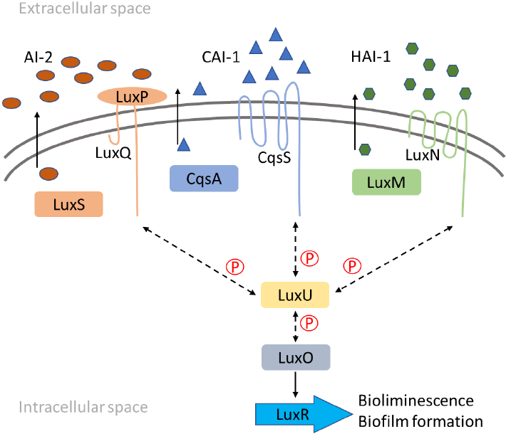
The QS mechanism of V. harveyi has been well characterized and a brief description is presented in Figure 1. Briefly, V. harveyi uses three different signaling molecules, CAI-1, HAI-1, and AI-2, produced by the CqsA, LuxM, and LuxS proteins, respectively. These molecules freely cross the cell membrane and accumulate in the extracellular space till reach a threshold and are sensed by membrane proteins. Each signaling molecule has a cognate membrane protein, CqsS for CAI-1, LuxN for HAI-1, and LuxP-LuxQ for AI-2. Once sensed, the membrane proteins reduce the phosphorylation activity over the LuxU, and this, in turn, reduces the LuxO phosphorylation. This reduction activates the LuxR protein expression which represses and activates many genes, like genes related to the bioluminescence and biofilm formation [12- 14].
Mathematical model
In the V. harveyi QS mechanism three different AIs are produced and detected, nevertheless, to simplify our model, we only considered the AI-2 dynamic. Our model was made based on the next assumptions i) the AI-2 production by the LuxS synthase is dependent on cell growth [15]; ii) it is considered that all produced AI-2 freely cross the membrane to the extracellular space.
The V. harveyi QS model is composed of the Gompertz function to adjust the V. harveyi growth curve (X), and the extracellular AI-2 concentration (A). The model is described as follows:
The bacterial growth dynamic is described using a Gompertz function in Equation (1), where X 0 is the initial bacterial concentration, C is the asymptote of the function, and represent the maximum bacteria concentration, B is the slope of the function which represents the growth rate, and M is the saturation time.
Equation (2) describes the A dynamics, μA is the AI-2 synthesis. μXA is the uptake of A by the bacteria. μA is presented below.
where kA is the A velocity production, and km1 is an affinity constant. The uptake of A is described by a function μXA as follows:
where kXA is the uptake rate by the bacteria, and km2 is an affinity constant.
Parameter estimation
Parametric estimation of the mathematical model can be understood as the search of values for parameters set (θ) that minimize the difference between the model outcome y i and experimental data y i as close to zero as possible. This search is restricted by the system dynamics, algebraic restrictions and systems constraints. Focused on this aim, the Sum of Square of Weighted Residues (SSWR) has been used successfully in others works as cost function [10],[16] [17], and is defined as follows.
where j and i represents the number of variables and experimental data, respectively, y is the set of experimental data points, and y is the model outcome. Since the integration routine of Equation (2) requires dense data sets at different times depending on adaptive step size, inputs in each estimation are approximated by a linear interpolation. The minimization of Equation (5) implies a nonlinear optimization problem with several variables that can be solved using a global optimization algorithm. In this work, we used the Differential Evolution (DE) algorithm [18] to estimate the optimal parameter values.
Parameter identifiability
A parameter is identifiable if can be determined by a value within a confidence interval with a desired probability. The parameter identifiability plays an important role for analysis of parametric models because the parameters define the model performance and its adaptability under different conditions [7],[19].
In order to analyze the parameter identifiability in Equations (1) and (2), we used the approach based on the profile likelihood presented by Raue et al. [7]. This approach offers insights into the parametric identifiability. Additionally, this approach explores the practical and structural non-identifiability, two phenomena related to parameters.
Briefly, the approach consists on defining a set of values for each parameter, centered at its optimized value, and re-optimize the remaining parameters minimizing the SSWR[7]. The objective of this approach is to explore the parameter search space around the optimal value of each parameter, while the model outcome is re-optimized estimating the remaining parameters [9].
Parameter uncertainty and dependency
Due to the stochastic nature of biological systems, when a mathematical model that describes a biological phenomenon is developed, is necessary to consider the data variability. Additionally, the measuring methods normally add noise to the measurements, incrementing the data variability. The bootstrap method is a statistical tool to determinate the parameters accuracy and parameters dependency.
For parametric bootstrap is necessary to know the data distribution, which is normally unknown. To tackle this issue, the weighted bootstrap method assigns to the cost function a vector of random weights from an exponential distribution with mean and variance one [8]. This method has been used successfully in others similar works [9],[10]. In each weighted bootstrap repetition, the model parameters are re-optimized, and after enough repetition, the confidence interval is calculated. The 95% confidence interval for each parameter is calculated between the 2.5 and 97.2% quantiles. From the confidence interval, the distributions of parameters and dependency among parameters are plotted.
NUMERICAL RESULTS
Initially, the parameters were estimated to find a set of parameters values that adjust the model outcome to experimental data. The experimental data were taken from [14], using the Plot Digitizer program to obtain the numerical data from the graphics [20]. Because the growth function is independent, firstly we estimate the growth function parameters and used the best fit values as constants for estimations of remaining parameters. The best fit values of growth function parameters are presented in Table 1.
Table 1. Parameter values of the growth function. These values are fixed in further estimation.
| Parameter (units) | Best fit |
|---|---|
| X 0 (OD 600) | 0.00091 |
| C(OD 600) | 3.2357 |
| B(t) | 0.3514 |
| M(t) | 10.7743 |
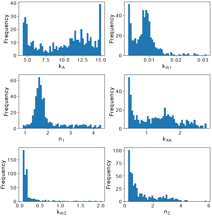
The remaining model parameters were estimated using the values in Table 1, and the best fit value set was used to calculate the profile likelihood [7], this method has been successfully used in previous similar works [9],[10]. For each parameter, a vector is defined with values centered at its best-estimated value and use to explore its parameter space. The profile likelihood results can be seen in Figure 2. The graphics show a concave shape that means there is a parameter value that minimizes the model error, and the model parameters are identifiable.

After identifiability analysis, we perform the weighted bootstrap method to analyze the parameters uncertainty and parameter dependency and compute the confidence interval. Firstly, 500 weighted bootstraps repetitions were made, re-optimizing the parameters on each repetition. Then, the 95% confidence interval was calculated, using the 2.5 and 97.5% quantiles, and the intervals are presented in Table 2.
Table 2. Parameters confidence interval and best fit.
| Parameter (units) | Best Fit | Confidence interval | |
|---|---|---|---|
| 2.5% quantile | 97.5% quantile | ||
| k A (μM⸳t -1) | 4.6361 | 4.3507 | 15.0 |
| k m1(OD 600) | 0.0025 | 0.0021 | 0.0312 |
| n 1 | 3.5412 | 0.8991 | 4.3129 |
| k XA (t -1) | 0.4769 | 0.4477 | 2.7818 |
| k m2 (OD 600) | 0.1674 | 0.0704 | 1.9998 |
| n 2 | 3.0957 | 0.2375 | 5.8004 |
Parameter kA is the parameter with the larger interval confidence. On the other hand, km1 has the smaller interval confidence of all parameters. That means, kA can variate along a long interval and the model is still suitable, but the smaller interval confidence of k m1 means that the model is more sensible to it. Based on the confidence interval, the distribution of parameters is depicted in Figure 3.
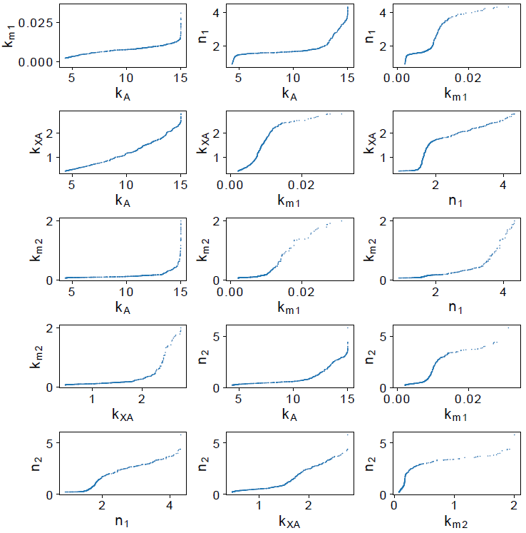
In Figure 4, parameters kA and kXA show a linear dependency, increasing the value of kA , the estimation of kXA also increases. These parameters can not be estimated independently. This behavior is consistent with the real system, if the velocity production of AI-2 (kA ) increases, is necessary that the AI-2 uptake rate (kXA ) also increases to balance the extracellular AI-2 concentration.
To improve the parameter estimation, one of these parameters must be fixed for further estimations. This approach has been successfully used to reduce the parameter estimation process, which helped to reduce the computational cost and improves the model fit [10]. In this work, they fix the parameters based only on the profile likelihood because they found that some parameters were structurally non-identifiable. In our work, profile likelihood of all parameters showed that all parameters are identifiable, but parametric dependency analysis showed up that some parameters are dependent on each other. Fixing a dependent parameter helps to improve the model fit and to reduce the parameters confidence interval [9].
Using this approach, we fixed k XA =0.4769 for further estimations and to analyze the remaining model parameters. The selection of k XA as the fixed parameter was to analyze the impact of this approach in a parameter with a large confidence interval. Once k XA fixed the likelihood of remaining is computed, and the graphics are depicted in Figure 5. There is a remarkable improvement in the identifiability of most of parameters. Confidence interval, parameter distributions and dependency among parameters were re-calculated after a new set of 500 weighted bootstraps repetitions. The confidence interval and best fit parameters value are depicted in Table 3.
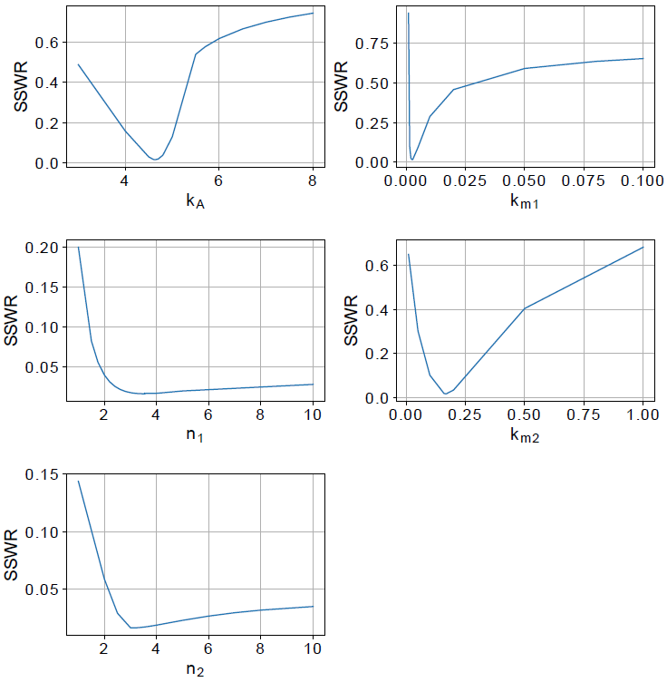
Table 3. Parameters confidence interval and best fit value after estimations with kXA fixed. *means that parameter was fixed in estimations.
| Parameter (units) | Best Fit | Confidence interval | |
|---|---|---|---|
| 2.5% quantile | 97.5% quantile | ||
| k A (μM⸳t -1) | 4.6361 | 1.8900 | 4.6649 |
| k m1(OD 600) | 0.0025 | 0.0001 | 0.0072 |
| n 1 | 3.5412 | 0.2023 | 4.4556 |
| k XA (t -1) | 0.4769* | ||
| k m2 (OD 600) | 0.1674 | 0.1582 | 2.5 |
| n 2 | 3.0957 | 0.8611 | 4.1206 |
Remarkably, the best-fit values are the same as that of the previous estimations. Fixing the parameter k XA does not affect the parameter estimation but reduce the computational cost and improves the confidence interval.
Also, the estimated parameters get a distribution more defined, as can be seen in Figure 6, where the parameter k A varies less when parameter k XA is fixed.
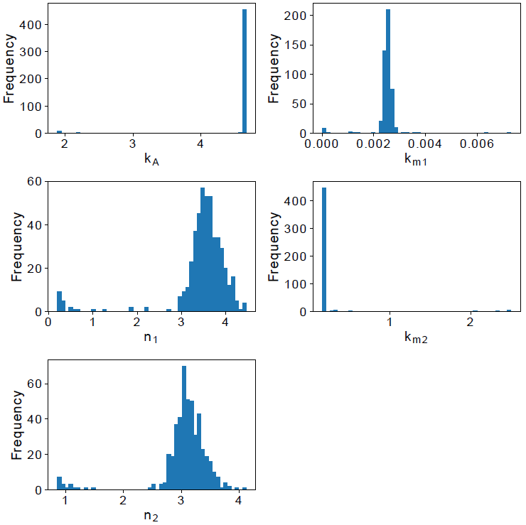
Figure 6. Graphs of the parameter distribution after fix parameter kXA in weighted bootstrap repetitions.
The reduction of confidence interval also improved the parameter distribution, which is visually evident in parameters kA , km1 , and km2 in Figure 6.
Nevertheless, as in Figure 3 there is one tail distribution in parameters, which could be attributed to the estimation method used is stochastic and its random nature.
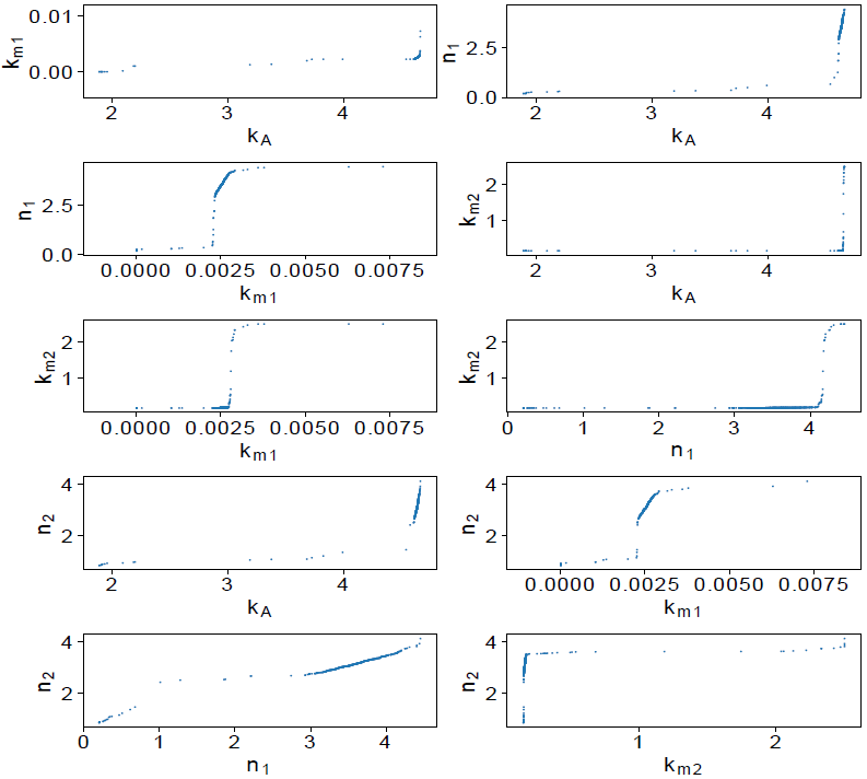
The parameter dependency is presented in Figure 7. Parameters n 1 and n 2 present a behavior like parameters k A and k XA , which seems to be dependent. Nevertheless, based on their distribution (Figure 6) and confidence interval, we considered that the parameter dependency is not significative to affect the model performance or parameters identifiability. After parameter analysis, we consider that by fixing k XA the remaining parameters are identifiable.
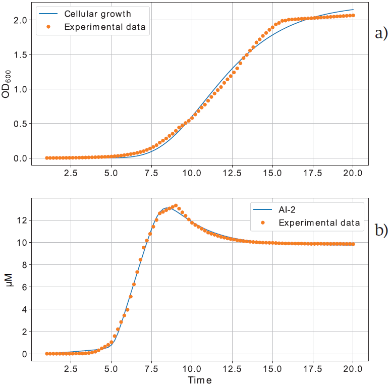
The model performance is presented in Figure 8, the model outcome in blue lines, and experimental data in closed circles [14]. Parameters values are presented in Table 1 for Equation (1), and Table 3 for Equation (2). As can be seen, the model presents a good performance to adjust the experimental data, despite there are misalignments when the experimental data change drastically, about the hour eight for AI-2 dynamics, and hour 15 for the cellular growth.
CONCLUSIONS
In this paper, we presented a mathematical model that describes the AI-2 dynamics as a function of the bacterial growth in the V. harveyi bacteria, and the model viability was probed by the parameter identifiability analysis as can be seen in Figure 8, our model can represent adequately the experimental data from [14].
Despite the identifiability analysis showed that all parameters were identifiable, the parameter dependency analysis showed that kA and kXA were dependents, additionally, the dependent parameters do not present a clear distribution.
Despite both parameters are identifiable, they can increase or decrease arbitrary without enhance the model adjustment.
Fixing kXA , the identifiability and confidence interval of remaining parameters was improved and the distribution of kA showed a clear tendency to a centered value. This is a new way to tackle the identifiability problem and enhance the model parameters viability.
As future work, we propose a deeper analysis about the influence of bacterial growth on the AI-2 dynamics. Additionally, further analysis can be realized for a better understanding about the effect of a dependent parameter over the other, this could be useful to controls the parameters tendency, which can mean a saving of resources during the experiments.

