


 nueva página del texto (beta)
 Inglés (pdf)
 Artículo en XML
 Referencias del artículo
 Enviar artículo por email
 Citado por SciELO
  Similares en
SciELO
Similares en
SciELO 
 Permalink
INTRODUCTION
From the time of Aristotle the analysis of human movement has been of interest to mankind [1]. The first formal studies on human gaits were made at the end of XIX century. Initially human gait analyses were performed by a set of photographic cameras sequentially activated to follow the motion. However at the end of World War II the first laboratories for human motion analysis were created [2]. By means of processors, video cameras and lighting techniques these laboratories were able to obtain human motion data. Nowadays there are several measuring and tracking systems cable of capturing 3D kinematic and kinetic human gaits. Most of these systems are based on visual observations by means of optical devices such as video cameras and photography. An example of tracking systems is the CaTraSys (Cassino Tracking System) [3], a cable-based parallel manipulator used to obtain experimental data of human walking characteristics. Three-dimensional motion analysis has been also performed by using the VICON System for data capture [4] [5] [6]. Measuring and tracking systems can be also combined with biomechanical modelling to study, analyse and predict human motion[2].
Tracking systems also measure human 3D gaits by mean of different type of sensors (accelerometers, optoelectronic, magnetic, etc.), which can be wireless or cable-based. With the assistance of computer technology in the 1970s, trunk acceleration amplitude and rhythmicity were used to discriminate between healthy individuals and different types of walking pattern, such as crutch assisted gait, peripheral nerve injury, post-operative hip arthroplasty, and below knee amputees. In the same decade, spatiotemporal variables such as lower limb segmental velocities, heel strike, foot flat, heel off and toe off were also calculated from accelerometer data. More recently, it was demonstrated that accelerometers can provide useful insights into the motor control of normal walking, age-related differences in dynamic postural control, and gait patterns in people with movement disorders [7].
Visual analysis of human motion has become a major application area in computer vision. This development has been driven by many interesting applications and the recent technological advances involving the real-time capture, transfer, and processing of images on widely available low-cost hardware platforms. Functionality and performance is likely to be gained by adding a symbolic component on top of the image processing to reason about the scene and control image tasks. Work on different sensor modalities (range, infrared, sound) will also lead to systems with combined strengths [8]. A review describing the reliability of three-dimensional kinematic gait data was presented in [9]. This review provided evidence that clinically acceptable errors are possible in human gait analysis.
This paper presents the analysis of human gait of three young adults under walking conditions similar to those in real life. The aim is to determine how the human gait varies under different conditions. The walking conditions considered in this study are: ascending a slope walk, no arm-swing walk, carrying a front load walk, carrying a lateral load walk, and high-heel shoes walk.
RELATED WORKS
In the last three decades, there has been several research works focused on the understanding, analysis and characterization of human gait. These research works can be classified into two main groups: study of human gait of non-disabled people (healthy people) and study of human gait of disabled people. The following paragraphs summarize some of these works.
Human gait of non-disabled people
It has been reported that walk ratio remains invariant except at slow speeds [10] [11]. On the other hand, a kinematics and kinetics gait analysis of children showed that repeatability of kinetics data was higher than kinematics data [5]. A study of gait acceleration and synchronisation in healthy adult subjects was presented in [12]. A model equation with two parameters that capture the essential relationships between gait cycle and gait acceleration was derived. In [13] the repeatability of gait parameters measured by a force plate gait analysis system (Leonardo Mechanograph® GW) in healthy children was analysed. A comparison of lower extremity coordination in walking and running was reported in [14]. An investigation presented in [15] demonstrated that walking speeds using Froude number fractions below one is a method to establish dynamic walking similarities between different subjects. In [16] it was found that gait patterns are not a fixed patient characteristic, but often vary with walking speed. An investigation showed that kinematics walking pattern of 6 year-old girls and 18 year-old girls have small differences between the two groups of girls [17]. Walking pattern with missing-heel shoes differs drastically from the pattern with normal sole geometry in the sagittal plane during the first half of the gait cycle [4]. In [18] it was found that individuals should be given at least 5 min of walking or other normal activity to adapt to altered inertial conditions before gait assessment is conducted. On the other hand, in [19] it was found that visual condition, particularly double and tunnel vision, in healthy elderly influences gait characteristics and interacts with gender.
More recently, an investigation to examine how different modes of arm swing affect gait stability was presented in [20]. Ten healthy young male subjects were asked to walk with four different arm swing instructions at seven different gait speeds. The results evidenced that excessive arm swing significantly increases local dynamic stability of human gait. On the other hand, a study of human gait transitions and functional distance on a treadmill was presented in [21]. The results showed that the increase of functional distance reduced the amount of classical hysteresis and promoted negative hysteresis, that is, a lower transition speed forwalk-to-run transitions (ascending trials) than for run-to-walk transitions (descending trials). An evaluation of the human gait phase resetting response of healthy individuals when perturbing the right leg was presented in [22]. The results showed that phase resetting behaviour is relatively consistent among subjects, but that minor variations in phase resetting behaviour are attributable to walking at different treadmill speeds.
Human gait of disabled people
An investigation to analyse the regularity and complexity of the Minimum toe clearance time series due to healthy ageing and locomotors' disorders was conducted [23]. The results suggested that ageing influences gait patterns which in turn can affect the balance control of human locomotion. A study to analyse the variation of gait patterns after surgery to repair an anterior cruciate ligament rupture, and to investigate the effect of knee bracing was reported in [24]. The results revealed that patients treated with a brace showed remarkable differences in walking patterns compared to those patients treated without a brace. In [25] it was found that experienced amputees have better walking performance than their relatively prosthetic inexperienced counterparts. On the other hand, in [26] it was observed that the overall walking pattern in children treated for clubfoot was good despite smaller persistent deviations from normal. In [27] it was observed that doing sports in the youth has effects on movement patterns (smaller changes in the angle of the ankle joint) in all day living.
Git patterns of neurologically healthy adults do not necessarily result in faster gait speeds for individuals with chronic stroke [28]. The effects of auditory rhythms and arm movement on inter-segmental coordination during walking in persons who have suffered a stroke were studied in [29]. An investigation to estimate 3D femoral and tibial linear accelerations during treadmill walking on healthy and osteoarthritis populations was presented in [30]. Kinematic and kinetic characteristics of walking pattern for patients with cerebral palsy (CP) were investigated in [31]. In [32] it was found that the use of the peroneal nerve stimulator in hemiplegic patients does not introduce any excessive and potential harmful mechanical loads. Alternatively, in [33] it was observed that the reproducibility of walking patterns differs between patients with arthrogryposis multiplex congenital and a healthy control group. The emergence of muscle activity pattern during walking in toddlers with typical development (TD) and with Down syndrome (DS) was studied in [34].
From this literature review it can be observed that human gait analysis has been mainly focused on the characterization of healthy and pathologic gaits during normal free walk conditions. Several works report the variation of gait patterns to walking speed. However, very few works have considered the analysis and characterization of gait profiles under different walking conditions as they may usually occur in real life situations; for example, ascending a slope, walking with high-heel shoes, walking while carrying a load, etc. Under these real life conditions human gait may vary and therefore this variations should be considered when providing diagnosis, defining rehabilitation procedures, or designing prosthesis or equipment in order to obtain more robust designs.
This research work presents the analysis of human walking patterns of three young adults under normal and especial conditions such as walking with and without arm swing, ascending a slope, fast walk, slow walk, with a front load, etc. The objective is to compare and evaluate gait variations corresponding to different real life walking situations. A set of kinematic gait parameters is defined and used to evaluate and analyse human gaits. Human gaits are reconstructed by a 3D computer vision system.
METHODOLOGY
Reconstruction methods
In order to determine the most suitable computer vision method to reconstruct the 3D gait trajectories, an evaluation of the most common 3D reconstruction methods in the literature was conducted. These methods are:
The linear method based on the homogeneous solution of the calibration matrix, by singular values decomposition (SVD) [35] [36].
Linear method based on the non-homogeneous solution of the calibration matrix, [35] [36] [37] [38] [39].
Non-linear method called Camera Space Manipulation (CSM) [40] [41], using an iterative process
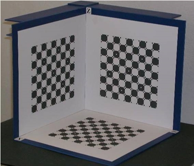
The first two methods require a camera calibration process to determine the intrinsic and extrinsic parameters of the camera. In this process the projection matrix P, also called calibration matrix, is estimated and then the intrinsic and extrinsic parameters of the camera are obtained. The estimation of the projection matrix P can be made by a known scene such as a calibration pattern made of three planes [35] [36], Figure 1.
Homogeneous solution of the calibration matrix
This method solves the calibration matrix by using the SVD of the equations that projects a point from the 3D world to the camera image plane [35], [38]. A projection matrix from which all intrinsic and extrinsic parameters can be extracted is obtained. A camera generates 3D (X i ) point correspondences, with points in the image plane (x i ). If there are enough X i <->x i correspondences, a camera matrix P can be estimated as:
where X i corresponds to the 3D coordinates and x i corresponds to the coordinates in pixels. The size of matrix P is 3×4 because each 3D point has four homogeneous components (X, Y, Z, 1)T, and the point on the image plane has three homogeneous components (x, y, 1)T. The solution P is obtained by SVD using Matlab®.
Non-homogeneous solution of the calibration matrix
Assuming that there are point correspondences
which involves 12 unknowns. Since the non-homogeneous solution will be used, the element
Camera Space Manipulation (CSM)
The Camera Space Manipulation method is a computer vision technique that does not require a calibration process [41], [42]. An important feature of this method is that the manoeuvring targets are defined and pursued in the reference frame of 2D images obtained by each of the participating cameras; in this case two cameras. These targets are established using "six vision parameters", which are determined by a nonlinear estimation process called "least squares differential correction". These parameters define a nonlinear algebraic relationship between the internal configuration of a robot and the corresponding location in the camera space of visual marks placed on the manipulable body. A simplified pin-hole camera model is obtained by considering the asymptotic limit when Zo is much greater than the other coordinates x i , y i , z i , X o and Y o , [9]. Then, the coordinates in the image plane (xci, yci) are:
These equations define the orthographic camera model, where C1,…,C6 represent the vision parameters that define a nonlinear algebraic relationship between the physical location of 3D points (x i , y i , z i ) and the corresponding location in the image plane (x ci , y ci ). To determine the six vision parameters the same calibration pattern used in the two previous methods is used. Six parameters are determined independently for each camera. Since Eq. (3) is nonlinear in terms of the vision parameters, the estimation process is iterative and can be derived from the nonlinear estimation process called "least squares differential correction".
The values of the vision parameters were obtained using Matlab®, and the equations obtained are:
where the [X, Y, Z] vector corresponds to the spatial coordinates of the point.
Evaluation of vision reconstruction methods
To quantify the accuracy of each reconstruction method, the calibration pattern was used. Three test points were selected, the furthest in each plane. These points are presented in Table 1, together with their corresponding coordinates, in pixels, for each camera.

The 3D reconstruction of the test points was performed using the three different methods. The results are shown in Table 2. To determine the reconstruction error, the following criteria was used:

where
Data processing
Having selected the reconstruction method, it is necessary to define the methodology to carry out the image processing and obtain the coordinates of the markers (centroids) placed on the person under analysis. In this study six white circular markers were located at each individual’s leg, Figure 2a. The ankle and end of femur were defined by markers on the lateral malleolus (marker 2 and 4). Markers 1 and 3 were located at the thigh and tibia, respectively. Marker 5 was located at the heel and marker 6 at the metatarse before the phalanges.

FIGURE 2 Image processing: a) markers location at individual’s leg, b) image obtained from the video, c) image converted to a grey scale, d) binarized image, e) location of the centroids.
The following equipment was used to carry out the 3D reconstruction:
›Two cameras uEye UI-1640-C.
› Two tripods for cameras.
› A calibration pattern of three planes.
› Dark clothing for individuals.
› Dark curtains.
› White circular markers.
In order to obtain the videos to reconstruct the human gait trajectories, a stage was set up as shown in Figure 3. The two cameras were placed equidistant with respect to the main axis of the stage, and they were focused to have an adequate view of at least three steps. The calibration process was performed by locating the calibration pattern at the central step of the stage and at an average altitude between the highest and the lowest markers placed on every person (marker 1 and marker 6, respectively).

Once a video has been obtained with the cameras, it is defragmented into images which are then processed. The image size used was 1024 x 1280 x 3 pixels, Figure 2b. Each image is converted to a grey scale image, Figure 2c. Then the image is binarized using a threshold value to separate the objects of interest, Figure 2d.
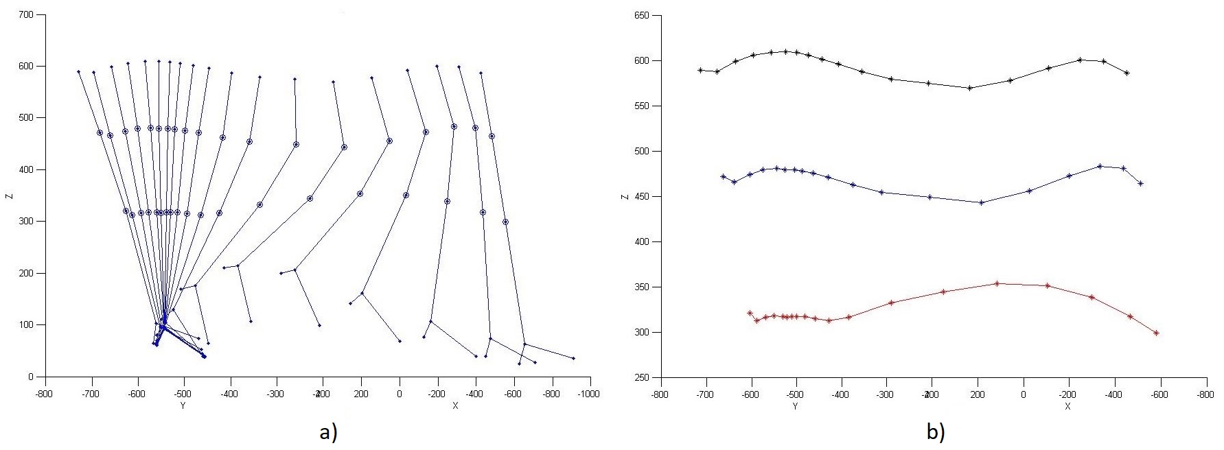
Once the image has been binarized, the centroid of each marker is computed according to the algorithm shown in Figure 4. The results are shown in Figure 2e. After obtaining the coordinates of the markers in the 2D camera space, they are transformed to the 3D real world space as shown in Figure 5a. In this way, 3D trajectories describing the human walking movement can be obtained as shown in Figure 5b.


Once the image has been binarized, the centroid of each marker is computed according to the algorithm shown in Figure 4. The results are shown in Figure 2e. After obtaining the coordinates of the markers in the 2D camera space, they are transformed to the 3D real world space as shown in Figure 5a. In this way, 3D trajectories describing the human walking movement can be obtained as shown in Figure 5b.
Three young adults, two men and a woman, aged 20-30 years old, were considered in this study. They were neurologically and orthopedically intact, and with the corporal characteristic as shown in Table 3. Informed consent was obtained from all the subjects. Since the main objective was to investigate if the human gait varies under different walking conditions, a sample of 3 subjects was considered appropriate at this moment.

Experimental procedure
From a preliminary study the most common real life human walking conditions were identified as follows:
› Ascending a slope walk (AASW)
› Horizontal walk (HW)
› Arm-swing walk (ASW)
› Not arm-swing walk (NASW)
› Carrying a front load walk (CFLW)
› Carrying a lateral load walk (CLLW)
› Not load walk (NLW)
› Slow free walk (SFW)
› Fast free walk (FFW)
› High-heel shoes walk (HHSW)
› Not high-heel shoes walk (NHHSW)
Thus, the subjects were asked to walk along a straight walkway according to these conditions. Each person performed several attempts for each condition to discard unnatural behaviour. Video was taken for each person and condition.
Gait parameters
Several kinematic gait parameters were defined in order to quantify and analyse walking patterns. It has to be mentioned that although most of these parameters have been used in the literature, they have been measured in 2D while in this paper they are measured in 3D.
Angle between femur and tibia
The angle between the femur and tibia, Θ, defines the angular amplitude of the knee flexion movement. This angle can be computed as follows:
where a, b and c are the distance vectors between markers 2 and 3, 1 and 3, and 1 and 2, respectively.
Step amplitude
This parameter refers to the step length, i.e. the distance from the instant where the foot touches the ground until it touches the ground again after the swing phase. This parameter is also considered in several research works, e.g. [27]. In order to calculate the step length, marker 4 was used as reference. The step amplitude can be calculated as:
where L is the step amplitude.
Cycle time
The cycle time corresponds to the time required to perform a complete gait cycle, as it is widely used in the literature, e.g. [18], [19]. The cycle time is calculated by the total number of frames in a gait cycle and the time elapsed between frame and frame. In this case the time between frame and frame is 0.02 s. Thus, the cycle time is calculated as:
where T is the cycle time and N F is the number of frames in the complete gait cycle.
Step height
The step height parameter refers to the maximum elevation of the foot relative to the ground during walking. This height is computed as the difference between the maximum and minimum Z coordinates during a complete gait cycle:
To obtain the Z coordinates, marker 4 is defined as the reference.
Deviation between tibia and femur
In the literature it is mentioned that the knee has a second degree of freedom which corresponds to a rotation relative to the longitudinal axis of the leg. However this effect is only qualitatively described without any quantification. In order to quantify this effect, a new parameter is defined based on the maximum deviation between the tibia and femur (Δd). The relevance of this parameter is to evaluate the second degree of freedom of the knee, which may be considered in the design of transfemoral prosthesis.
The deviation between tibia and femur parameter refers to the maximum distance between marker 3 (on the tibia) and marker 2 (on the end of femur), measured from a top view of the 3D trajectory and considering the sagittal plane as reference. To estimate Δd the difference between the distances d 1 and d 2 is considered, see Figure 6:

where d 1 corresponds to the maximum distance and d 2 is the average distance between marker 3 and marker 2, at the zone where these markers remain parallel.
RESULTS
The results of the 3D gait pattern analysis under different conditions are presented in Table 4. For each person and walking condition, the human gait parameters were calculated and analysed.

Knee flexion amplitude
From Table 4 it is observed that model 1 (woman) had the largest amplitude of knee flexion, from 118.6° to 172.7°, i.e. an amplitude of 54.1°. The average knee flexion amplitude was 44.8°.
Step amplitude
There is a relationship between the height (Table 3) of each subject and the step amplitude (Table 4). The tallest subject (1.72 m) showed the largest step amplitude (1085.7 mm). On the other hand, model 1 (the shortest model) had the smallest step amplitude (977.1 mm). The step amplitude of subject 1 under the HHSW condition increased from 977.1 mm to 1037.3 mm, which is greater than her average value.
Cycle time
Regarding the cycle time, an average cycle time of 0.42 s was obtained, which is in agreement with the values reported in the literature [5], [10], [11], [14], [16]. Model 1 (woman) registered the shortest cycle time, 0.40 s.
Step height
An average step height of 59.5 mm was obtained. However, in the case of model 1 under HHSW condition, the step height was 37.2 mm, which corresponded to the smallest value and represents the 62.5% of the general average value. This suggests that it represents a high risk of tripping when walking on irregular terrain when high heels shoes are used.
Deviation between tibia and femur
The general average value of the maximum deviation between tibia and femur was 15.4 mm. Considering an average distance of 167.1 mm between markers 2 and 3 (end of femur and tibia), an angle of 5.3° will produce this average deviation between tibia and femur. This angle corresponds to the rotation angle of marker 3 (on tibia) with respect to the sagittal plane. Due to the small magnitude of this deviation angle, it is commonly assumed that the movement of the tibia and femur are only on the sagittal plane.
Foot movement
It was observed that at the stance phase (first 10 frames), when the foot supports the entire body weight, the foot takes a different morphology than when it has no load (swing phase), see Figure 7. This is deduced by estimating the distances between the ankle and heel (markers 4 and 5), the ankle and metatarsals (markers 4 and 6), and the heel and metatarsals (markers 5 and 6). These distances are estimated from the 3D reconstruction and they are almost the same at the stance phase, but different during the swing phase. This results evidence that the foot changes its pose during the gait cycle.

Femur and tibia movement
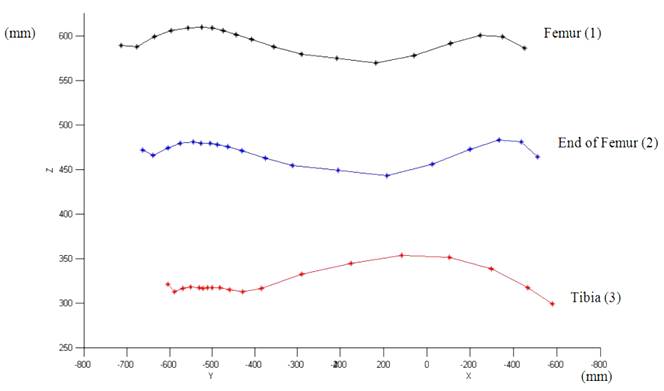
The trajectories described by markers 1 and 2 are very similar in terms of shape, as it was expected, see Figure 8. However marker 3 generates an inverse trajectory to trajectories of markers 1 and 2.
Knee flexion and leg shortening
In all subjects it was observed that the magnitude of the vector that goes from marker 2 to marker 3 (end of femur and tibia), is not constant and decreases with the leg flexion. The maximum variation of this vector (shortening) was 29.79 mm for subject 1, 27.89 mm for subject 2, and 25.51 mm for subject 3; showing an average shortening value of 27.73 mm. This value represents the average distance that the leg naturally shortens due to the knee joint and that prevents tripping during walking. The leg shortening effect is very important when analysing the knee joint and when designing knee prosthesis.
DISCUSSION
Walking on a slope
A ramp with a 6° slope was used to carry out the AASW tests. This slope represents the average value according to the information found in terms of regulations in Mexico and other countries [43]. The results have shown that in the AASW condition the cycle time and the deviation between tibia and femur parameters were greater than in the HW condition. On the other hand, the step amplitude, knee flexion amplitude, and step height parameters were smaller in the AASW conditions than in the HW condition. Figures 9 and 10 show the walking trajectories corresponding to the HW and AASW conditions, respectively.

Walk with and without arm swing
Figure 11 shows the trajectories described by markers 1, 2 and 3 for ASW and NASW conditions. From this figure it can be observed that NASW produced a slightly variation of the gait pattern, in particular markers 2 and 3 showed greater elevation than ASW trajectories. Figure 12 shows the knee flexion amplitude and the step height variation along a complete walk cycle for the ASW and NASW conditions. From this figure it is observed that the NASW condition requires a longer cycle time and produces smaller step amplitudes but with greater elevation than the ASW condition. The values of the maximum deviation between tibia and femur, the knee flexion amplitude and the step height parameters, were greater in the NASW condition than in the ASW condition. This suggests that NASW presents some instability that causes a slightly distortion of the natural gait pattern. Also NASW is slower than ASW and produces smaller step amplitudes.


Walking with or without a load
In this test the subjects were asked to walk with a pair of dumbbells, one in each hand. Each load was 5 kg for male and 4 kg for female. The results showed that the CLLW conditions led to the greatest cycle time, i.e. the slowest gait cycle. The values of the maximum deviation between tibia and femur and the step amplitude parameters were reduced when walking with a load, being the smallest values for the CFLW condition. In the case of the knee flexion amplitude and step height parameters, the values increased in the CFLW condition, Figure 13. Thus, it can be said that the human gait pattern is affected when carrying a load, leading to slower and shorter steps but with higher elevation than in the normal free walk.

Figure 14 shows the 3D walking trajectories of the HW, CLLW and CFLW conditions. From this figure it is observed that the HW and CLLW conditions describe a similar gait pattern, but in the CFLW condition the markers on the thigh and tibia tend to move to the right. This indicates that the human body adopts a different posture to maintain the balance when carrying a frontal load.

Slow and fast free walking
According to literature the normal walking cycle consists of three phases: the stance phase (50% of the cycle time), the swing phase (30% of the cycle time) and the double support phase of (20% of the cycle time). The results of the SFW condition are in agreement with these three phases and fractions. However, when a FFW condition occurs, the swing phase increases and the stance phase decreases, and as a consequence, the swing time increases and the support time decreases in comparison with the SFW. Figure 15 shows the 3D walking trajectories for the SFW and FFW conditions, where it can be observed that the amount of frames captured at the stance phase of the SFW conditions are greater than for the FFW condition. The values of the cycle time, deviation between tibia and femur, and knee flexion amplitude parameters were smaller in the FFW condition than in the SFW. The values of the step amplitude and the step height parameters were greater in the FFW condition than in the SFW condition, as shown in Figure 16.


Walking with high-heel shoes
The results of the HHSW condition (60 mm heel height) for subject 1 (woman) showed that cycle time for both HHSW and NHHSW (normal shoes walk) conditions are the same. However, the values of the maximum deviation between tibia and femur and the step amplitude parameters were grater in the HHSW condition than in the NHHSW condition. On the other hand, the knee flexion amplitude and the step height parameters decreased considerably in the HHSW condition. Figure 17 shows the walking 3D trajectories for the HSW and NHHSW conditions. From this figure it can be observed that the use of high heel shoes produces alterations in the sagittal alignment of the lower limbs and trunk. The markers on femur, end of femur and tibia, are very close to each other in the stance phase; i.e., the weight reception on the foot is not as gradual as with normal shoes.

From these results it is observed that the weight of a person is distributed on the foot, on both the anterior tarsal and posterior tarsal, approximately 50 %-50 %, but when high heels shoes are used the weight ratio increases on the anterior tarsal, altering the normal walk pattern and mechanics. A woman who wears high-heels shoes cannot step correctly, most of the weight falls on the forefoot and the effort comes to the knee in flexion. This is in agreement with the literature [44], [45], and is the cause of knee and back problems, dangerous falls, lower calf muscles, inflamed Achilles tendon, hammertoes, neuromas (benign tumors composed mainly of fibers and nerve cells), metatarsalgia (severe pain in the metatarsus of the foot), among others.
Human gait variation
Table 5 summarizes the effect of the different walking conditions on the human gait pattern for the three subjects under study. In this table the gait parameters corresponding to the each particular walking condition are compared with the gait parameters of normal walk, e.g. the AASW condition is compared with the HW condition. In this table the variation of the gait parameters are indicated as an increment (+), decrement (-) or equal (0) with respect to the reference normal walk. The gait variation is then described based on the variation of the gait parameters of the three participants when walking under a special condition in comparison with the gait parameters when walking under normal condition.

The results of the human gait analysis of the three subjects reveal that the human gait pattern varies with the walking conditions. In general, it can be said that the no arm-swing and the carrying a load walking conditions caused a slower walk with shorter steps and greater knee flexion and step height than the normal walk. On the other hand, the ascending a slope walking condition also caused a slower walk with shorter steps but with smaller knee flexion and step height. In the case of the fast free walking condition, the human gait was modified to produce larger steps with higher elevation but with a smaller knee flexion and deviation from the sagittal plane than normal walk. Walking with high-heel shoes produced larger steps with smaller knee flexion and step height than walking with regular shoes. It has to be mentioned that these results and observations correspond to the three subjects, and in the case of the high-heel shoes walking condition, the results correspond only to the female subject.
From the analysis of the 3D walking trajectories of the three participants under the different walking conditions, it has been observed that the variations of the human gait pattern are the result of a natural human reaction to compensate the variations of the human pose due to the special walking condition, e.g. carrying a front load, and to enhance the stability and equilibrium during such walking condition. Therefore these variations should be considered for medical diagnosis and orthopedics, pathological and aging evaluation, medical rehabilitation, and design of rehabilitation systems, human prostheses and humanoid robots.
Finally, it has to be mentioned that in order to provide more precise and standard quantitative results regarding the gait pattern variations under different walking conditions, the number of subjects must be increased considering different age, height, sex, weight, and health conditions of the participants.
CONCLUSIONS
An investigation to analyse the kinematic variations of the human gait pattern under several real-life walking conditions has been presented. For this purpose a computer vision system to reconstruct the 3D walking trajectories has been developed and presented. A set of gait parameters has also been defined in order to analyse and evaluate the human gait pattern variations. The experimental results of three subjects have revealed that human gait patterns vary with the walking conditions. It has also been observed that these variations of the human gait are the result of a natural human reaction to compensate the variations of the human pose and to enhance the stability and equilibrium during a particular walking condition. Therefore the variations of the human gait should be considered during the analysis, evaluation and diagnosis of gait performance, or during the design process of prostheses or rehabilitation systems.
Future work comprises an extensive statistically analysis of human gait variations comprising a large number of participants and with more walking conditions. Also future work considers the use of walking patterns and computer vision as a diagnosis tool in orthopedics for the analysis and evaluation of walking performance, and for the design of rehabilitation systems and prosthesis.

