


Serviços Personalizados
Journal
Artigo
 Inglês (pdf)
 Artigo em XML
 Referências do artigo
 Enviar este artigo por email
Indicadores
-
 Citado por SciELO
 -
 Acessos
Links relacionados
-
 Similares em
SciELO
Similares em
SciELO
Compartilhar

 Permalink
Revista mexicana de ingeniería biomédica
versão On-line ISSN 2395-9126versão impressa ISSN 0188-9532
Rev. mex. ing. bioméd vol.36 no.2 México Mai./Ago. 2015
https://doi.org/10.17488/RMIB.36.2.2pdf
Artículo de investigación original
On the Identification of an ICA Algorithm for Auditory Evoked Potentials Extraction: A Study on Synthetic Data
Identificación de un algoritmo ICA para la extracción de potenciales evocados auditivos: un estudio en señales sintéticas
N. Castañeda-Villa, E. R. Calderón-Ríos, A. Jiménez-González
Department of Electrical Engineering, Universidad Autónoma Metropolitana-Iztapalapa. México City, México.
Correspondencia:
Norma Castañeda-Villa
San Rafael Atlixco No. 186, Col. Vicentina. UAM-Izt, Edificio T
Cubículo 01. C.P. 09340. México, DF.
Correo electrónico: ncv@xanum.uam.mx
Fecha de recepción: 29 de noviembre de 2014.
Fecha de aceptación: 9 de enero de 2015.
Abstract
Extracting characteristics and information from Auditory Evoked Potentials recordings (AEPs) involves difficulties due to their very low amplitude, which makes the AEPs easily hidden by artifacts from physiological or external sources like the EEG/EMG, blinking, and line-noise. To tackle this problem, some authors have used Independent Component Analysis (ICA) to successfully de-noise brain signals. However, since interest has been mainly focused on removing artifacts like blinking, not much attention has been paid to the quality of the recovered evoked potential. This is the AEP case, where literature reports interesting results on the de-noising matter, but without an objective evaluation of the AEP finally extracted (and the influence of different implementations or configurations of ICA). Here, to study the performance of three popular ICA algorithms (FastICA, Ext-Infomax, and SOBI) at separating AEPs from a mixture, a synthetic dataset composed of one Long Latency Auditory Evoked Potential (LLAEP) signal and the most frequent artifacts was generated. Next, the quality of the independent components (ICs) estimated by such algorithms was measured by using the AMARI performance index (Am), the signal interference ratio index (SIR), and the time required to achieve separation. Results indicated that the FastICA implementation, with the symmetric approach and the power cubic contrast function, is more likely to provide the best and faster separation of the LLAEP, which makes it suitable for this purpose.
Keywords: synthetic auditory evoked potentials, independent component analysis, Amari performance index, signal interference ratio index.
Resumen
La extracción de características e información de los registros de Potenciales Evocados Auditivos (AEPs) es complicada debido a su baja energía, la que lo hace fácilmente enmascarable por artefactos de origen fisiológico o externo, como el EEG/EMG, el parpadeo y el ruido de línea. Este problema ha sido abordado por algunos autores mediante el uso del Análisis por Componentes Independientes (ICA, por sus siglas en inglés), que se ha utilizado principalmente para reducir artefactos. Estos trabajos han enfocado su interés en la tarea de remover artefactos como el parpadeo, por lo que han descuidado el estudio de la calidad del potencial evocado recuperado. Este es el caso del AEP, donde aun cuando la literatura reporta resultados interesantes en la reducción de artefactos, no existe una evaluación objetiva del AEP finalmente extraído (y el efecto de usar diferentes implementaciones/configuraciones de ICA). En este trabajo, con el objetivo de cuantificar el desempeño de tres algoritmos de ICA (FastICA, Ext-Infomax, y SOBI) en la calidad de la separación de los AEPs, se generó una mezcla sintética de señales compuesta por un Potencial Evocado Auditivos de Latencia Larga (LLAEP) y artefactos frecuentemente presentes en estos registros. Después, se cuantificó la calidad de los componentes independientes (ICs, por sus siglas en inglés) estimados por estos algoritmos utilizando el índice de desempeño (AMARI, por sus siglas en inglés) el índice de la relación de interferencia entre señales (SIR, por sus siglas en inglés) y el tiempo requerido para realizar la separación. Los resultados indican que FastICA, con el enfoque simétrico y la función de contraste potencia cúbica, proporciona la mejor y más rápida separación del LLAEP, lo que lo vuelve idóneo para esta tarea.
Palabras clave: potenciales evocados auditivos sintéticos, análisis por componentes independientes, índice de desempeño Amari, índice de la relación de interferencia entre señales.
INTRODUCTION
Event-related potentials (ERPs) are neurological responses obtained from EEG recordings result of periodic stimulation. In particular, when an acoustic stimulus is used, the response is referred to as the Auditory Evoked Potential (AEP), a signal that reflects the status of the neurological structures of the auditory system. These AEPs are originated in the cerebral cortex and can be detected by using scalp electrodes. However, due to the attenuation produced by the tissues in the path between the source generator and the recording point, the AEP amplitude is about ten times smaller than the EEG amplitude (10 μV versus 100 μV) [1]. As a result, the AEP is completely hidden by the EEG and easily overlapped by physiological (e.g. ECG and EMG) and environmental sources (e.g. line-noise) whose amplitude (many times larger than the AEP) and frequency content (similar to the AEP spectral components) make it impossible for conventional filtering procedures to extract the AEP.
Traditionally, the approach followed to extract the AEP aims to increase its signal to noise ratio (SNR) by attenuating the interference signals contribution. This is performed by the coherent averaging, a method that assumes that, while the EEG and other physiological signals remain uncorrelated and with zero-mean trial after trial, the AEP remains constant in amplitude and phase, which makes it possible to enhance it by averaging the trial-to-trial responses [2]. This is the most common strategy to deal with the low SNR, and it has been reported that the method may manage to increase it from a typical value of -26 dB to a value close to 6 dB [3]. However, in practice, it is well known that the coherent averaging has limitations due to (1) the natural change of the AEP, which may difficult the SNR enhancement, and (2) the large number of trials required to enhance the AEP, which involves the use of long-term studies (i.e. than 1000 trials) [3].
Alternatively, in an attempt to separate the undesirable sources, the EEG/ERP recordings have been decomposed by using Independent Component Analysis (ICA) [411]. In this approach, it is assumed that a group of p observations, x, measured by a set of sensors, can be modeled as a linear instantaneous mixture of q underlying sources, s, as

where x = [x1, x2, ···, xp]T, s = [s1, s2, ···, sq]T, and p ≥ q. Furthermore, the sources are assumed to be non-Gaussian (with zero-mean) and mutually statistically independent, which makes it possible for ICA to calculate a linear transformation W that, when applied to x, minimizes the statistical dependence of the output components and produces an estimation of the underlying sources (better known as the independent components, ICs), ŝ, as [12-13]

The recovered sources are statistically independent by definition, and results from different studies have appointed ICA as a compelling tool that, in consequence, has grown in popularity in the field of brain signal analysis [4-11]. Most of such works, however, have used ICA for de-noising purposes and, therefore, have focused on the estimates corresponding to the interference sources (e.g. eye movements) rather than on the estimates related to physiological events of interest like the AEPs. In addition, and because the original sources are unknown, only a small number of studies have paid attention to the identification of the ICA implementation that truly achieves an accurate recovery of such physiological events [4, 7, 10, 14].
The work described in this paper focused on the reliable recovery of Long Latency Auditory Evoked Potentials (LLAEPs) and presents a study that aimed to identify a suitable ICA implementation for such a recovery from EEG/ERPs recordings. To this end, the performance of three popular ICA algorithms for brain signal analysis (FastICA, Ext-Infomax and SOBI) and their configurations was tested on a synthetic EEG dataset. This by means of three indexes that evaluated (a) the overall quality of the ICA separation, (b) the quality of the LLAEP estimated by ICA, and (c) the time required to estimate the sources underlying the dataset.
METHODS
Synthetic data generation
The dataset was constructed by making two fundamental assumptions about the signals composing the EEG/LLAEP recordings: (a) the auditory response and the basal EEG are signals permanently present in these recordings and (b) the most common interference signals are the ECG, the blinking, the muscle activity, the electrode drift, and electrode noise.
The LLAEP appears at about 90 ms after the stimuli onset, lasts about 230 ms and, according to [15], can be generated by simulating an asymmetric biphasic complex (N100-P200). Thus, in this work, the positive half-period of an 8.25 Hz sinusoid was joined to the negative half period of a 6.25 Hz sinusoid, where the peak to peak amplitude of the LLAEP was fixed at 12 μV. Additionally, to keep a constant interval between consecutive potentials, the LLAEPs were generated at a rate of 1 Hz.
The basal EEG is a signal whose frequency content in normal conditions goes from very low frequencies (Delta-band, up to 4 Hz) to high frequencies (Gamma-band, 30-100 Hz). It is a permanent artifact that, unfortunately, cannot be avoided, reduced or eliminated during the LLAEP recording due to its physiological nature. Here, the EEG signal was produced using the generator available in [16], which made it possible to combine several sinusoids ranging from 0.1 to 125 Hz; with maximum amplitude of ± 20 mV.
Regarding the typical interferences, (a) the heart may produce electrical and mechanical artifacts in the EEG, and its presence indicates that an electrode is located on a blood vessel. In that case, the large amplitude and wide spectral content of the ECG turn the signal into a significant interference that affects both, the morphology and peak latency of the LLAEP waveforms. Thus, to take this artifact into account, this work produced a synthetic ECG by using the generator available in [17], with a frequency of 60 beats per minute and a maximum amplitude of 50 μV. (b) The blinking artifacts are produced by ocular movements that may be present even when the study is made in resting conditions, when the patient is lying, calmed and eyes closed. The eye blink is modelled by a "V" shape potential, which in this work was generated by a single triangular signal, with amplitude of 200 μV and randomly located in time [10]. (c) The muscle artifact is due to the muscle electrical activity produced by the contraction of either face muscles or muscles needed when swallowing saliva. The signal resembles spikes or a short burst activity, and it was generated here by using random noise (with amplitude of ± 200 μV) that was band-pass filtered between 20 and 60 Hz [5]. (d) The electrode drift artifact is caused by a lose electrode, and it was generated by a ramp in this work [10]. (e) Finally, to simulate electrode noise, an unfiltered white noise signal, with amplitude of ± 150 μV, was included in the dataset.
The synthetic signals and their corresponding probability density distribution (p.d.d.) are depicted in figure 1.

The EEG and the electrode noise signals have Gaussian distributions, the LLAEP, the blinking, the ECG and the muscular activity have super-Gaussian distributions, while the electrode drift has a sub-Gaussian distribution.
After the generation of each signal, a mixture was produced by calculating the product between them and a square matrix (A) that was randomly generated with values between -1 and 1 as reported in [18].
Separation into ICs by three implementations of ICA
To date, there are several implementations of ICA. Some algorithms are based on techniques that involve higher-order statistics (HOS), while others exploit the time structure of the sources to establish independence [8, 12, 13, 18-22]. Thus, while HOS implementations like FastICA [12, 18] and Ext-Infomax [21, 23] look for non-Gaussian distributions in the estimates, time structure implementations like SOBI [20, 22] look for no spatial temporal or no spatial time-frequency correlations.
These implementations can be easily downloaded from the webpages of the developers. However, to properly apply a particular ICA algorithm on a specific dataset, it is important to be aware of the criteria and parameters used by such an implementation to solve equation 2, otherwise the results may not make any sense. Such information will be described in the next paragraphs for the algorithms tested in this work:
a. FastICA (FICA) is a simple and relatively fast implementation to estimate independent sources from a linear mixture [12, 13, 18]. It estimates ICs by following either the deflation approach (Defl), where the components are extracted one by one, or the symmetric approach (Sym), where the components are simultaneously extracted. To work, it uses simple estimates of Negentropy (J), a very important measure of non-Gaussianity that, as shown in [12], can be approximated by means of the maximum entropy principle as

where w is an m-dimensional vector such as E{(wTv)2} = 1, v is a Gaussian variable with zero mean and unit variance and G is a non-quadratic cost function.
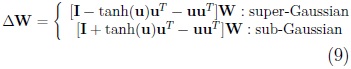
The problem is now reduced to find a transformation W whose vectors, w, are iteratively adjusted to maximize J (which is equivalent to reduce the mutual information). This is performed by a fixed-point algorithm that, in the deflation approach, is achieved by following the learning rule given by


and, in the symmetric approach, by the rule given by


where Diag (v) is a diagonal matrix with Diagaii (v) = vi, and g and g' are respectively the first and second derivative of G.
This ICA implementation converges much faster than gradient based methods, it is computationally simpler and requires little memory space, which turns FICA into a very popular implementation of ICA. However, the function g (commonly referred to as nonlinearity) must be carefully chosen to obtain a good approximation of the Negentropy and, therefore, of the ICs. Thus, commonly g functions used with the FICA algorithm include Tanh (i.e. g(v) = tanh(v)), Pow3 (i.e. g(v) = v3), Gauss (i.e. g(v) = v exp(—v2/2)), and Skew (i.e. g(v) = v2). Tanh is considered to be a good general purpose contrast function, while Pow3 is only recommended for estimating sub-Gaussian components when no outliers are present. (i.e. the algorithm performs kurtosis minimization), Gauss is useful when the independent components are highly super-Gaussian (or when robustness is very important) and Skew is recommended when high-skewness is characteristic in the sources.
In our study, the performance of FICA was tested on the simulated dataset using the entire set of combinations between the separation approach (i.e. Sym and Defl) and the nonlinearities (i.e. Tanh, Pow3, Gauss and Skew).
b. Ext-Infomax [21] is an extended version of the Infomax algorithm proposed by Bell and Sejnowsky [19], and makes it possible to separate sources with sub- and super-Gaussian distributions. To work, it uses a gradient based neural network whose algorithm can be derived by the maximum likelihood formulation that, in its logarithmic form, can be expressed as

where p is the hypothesized distribution of the sources, and the maximization of equation 8 is achieved by the modified learning rule given by
where the learning rules differ in the sign before the function tanh and are specified to the implementation by using a switching criterion as

where ki are elements of the N-dimensional diagonal matrix K and indicate the number of sub- or super-Gaussian distributions to be estimated by the algorithm.
In this work, the performance of this ICA implementation was tested when: (1) the algorithm automatically estimates the number of non-Gaussian sources (i.e. k=1) and (2) the user specifies the number of sub-Gaussian sources to be estimated by the algorithm (i.e. k= -1 since the simulated mixture included one sub-Gaussian signal, the ramp).
C. SOBI (i.e. Second-Order Blind Identification [20]) is an algorithm that defines independence by the absence of cross-correlations among sources and, thus, exploits their temporal structure to find W. To this end, SOBI performs the joint diagonalization of a set of several time-lagged covariance matrices, where the diagonalization of a matrix B can be represented as [22]

and the simultaneous diagonalization of k matrices becomes an optimization problem with respect to a matrix G such that the sum of all the off-diagonal terms in off (Bi), for i = 1, ··· ,k is minimum as

The diagonalizing matrix G turns out to be the mixing matrix A, from where it is possible to calculate W and thus, the ICs by using equation 2. Certainly, the key point on the performance of the algorithm is related to the number of time-delayed matrices specified by k. In fact, it has been reported that increasing this value makes the performance of SOBI more robust in poor SNR settings and less sensitive to large spectral overlapping between sources [20].
In this work, to test the performance of SOBI on the simulated dataset, three values of k were used to specify the number of time-lagged matrices to be diagonalized by SOBI: 100, 124 and 150. The former was used because it is the default value, while the latter two were used to cover respectively 50 % and 60 % of the total length of the epochs of the simulated LLAEP.
The combinations between the ICA implementations and the parameters tested in this work gave rise to a total of 13 configurations that are summarized in table 1.
Performance assessment
The performance of each ICA configuration was tested in three ways: first, by evaluating the overall quality of the separation, second, by evaluating the quality of the component of interest in this work, i.e. the separate LLAEP, and third, the time required to estimate the sources underlying the dataset. This was suitable due to the synthetic nature of the signals, which made it possible to use the Amari performance index (Am) to quantify the overall separation quality [24] and the signal to interference ratio index (SIR) to quantify the LLAEP separation [25]. Regarding the computational time, it was calculated using the Matlab© function cputime, which returns the CPU time used to execute a segment of code (the experiments were conducted in a computer with an Intel Core i5 processor (i5-3317U @ 1.70 GHz), 5.89 GB of RAM and Windows 8 Single Language).
In each case, the ICA configurations were applied ten times to the mixture, and the mean and standard deviation values of each index were finally calculated to quantify the stability of the decomposition achieved by ICA.
The indexes were calculated as follows:
a. Quality of the overall separation: Quantified by Am, it requires the knowledge of both, A and W to obtain a global matrix P = (pij) = WA from where Am is calculated as

where |pij| is the ij-th element of the matrix P, and the denominator is a normalization factor, i.e. the maximum value of the whole matrix. T hus, an Am value close to zero means that a good separation was achieved by ICA.
b. Quality of the separate LLAEP: Quantified by SIR, it requires the knowledge of a target signal to be compared against each of the ICs in order to quantify how much of such a target is present in them and, therefore, how well a specific source like the LLAEP could be estimated by ICA. In our case, the target signal was given by the synthetic LLAEP and the SIR index in dB was calculated by
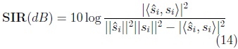
where ŝi is an IC, si is the target signal or pattern known, |<·, ·>| is the dot product, and ||·|| is the magnitude. In this way, the maximum value of SIR corresponds to the IC associated to the target signal (or at least to the IC containing the most of it).
RESULTS
Figure 2 illustrates the seven. ICs estimated by one iteration of the CA configuration that gave the largest mean value of Am, i.e. FICA-Defl-Skew. As expected, the separate signals have zero-mean, variance one and present the permutation and sign ambiguities typical of ICA., where the latter is evident in IC5 (the estimated EEG) and, after a careful observation , in IC7 (the electrode noise). Additionally, it can be seen that, while the blinking activity is clearly represented by IC1 and the ramp signal seems to be missing, the other simulated signals are present in more than one component. Thus, (a) some information of the muscular activity in IC2 is still mixed with the ECG in IC3 and the LLAEP in IC4, (b) part of the QRS information in IC3 is still mixed with the LLAEP in IC4, and (c) some electrode noise in IC7 and IC6 is still mixed with the EEG in IC5.

Figure 3 depicts the seven ICs estimated by one iteration of the ICA configuration that gave the smallest mean value of Am, i.e. FICA-Sym-Pow3. As before, the ICs have zero-mean, variance one and present both ambiguities, although the sign uncertainty is evident only in IC2, where the ECG was estimated with a negative sign. Regarding the separation, it can be seen that the number of mixtures is smaller than in the previous case, and that only IC6 seems to contain a combination of the ramp signal and some EMG and blinking activities. Thus, the electrode noise can be seen in IC1]-, the ECG in IC2, the muscular activity in IC3, the EEG in IC4, the LLAEP in IC5 and the blinking activity in IC7.
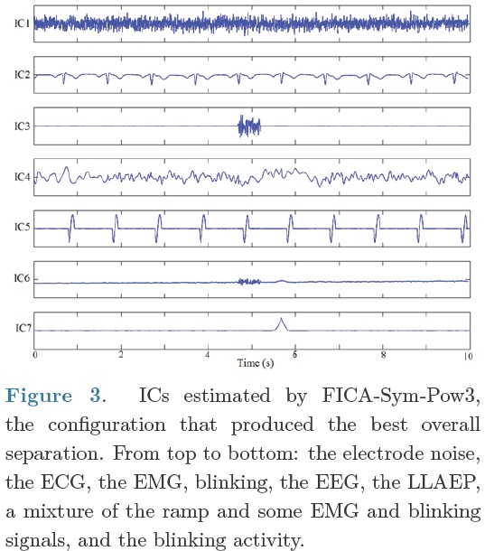
Figure 4 depicts the mean and standard deviation of the index used to evaluate the overall quality of the separation for the thirteen ICA configurations tested in this work (Am). In general, it can be seen that the Am index presented three behaviors, (1) mean values larger than 0.7 (enclosed by red circles), (2) mean values smaller than 0.7 with standard deviations smaller than 0.003 (enclosed by blue squares), and (3) mean values smaller than 0.7 with standard deviations larger than 0.038 (enclosed by green rectangles).

In particular, as indicated by the red circles (and summarized in table 2), independently on the approach selected, the configurations given by FICA-Skew produced the largest mean Am values , where FICA-Sym-Skew presented a value of 0.99 ± 0.003 and FICA-Defl-Skew presented a value of 1.1 ± 0.054. Regarding the configurations whose index; remained below 0.7, the blue squares indicate that the smallest values in both, mean and standard deviation were given by FICA-Sym-Pow3 (0.13 ± 0.000), Ext-Infomax-N-1 (0.16 ± 0.000), SOBI-150 (0.16 ± 0.00), Ext-Infomax-Ni. (0.16 ± 0.002), SOBI-124 (0.17 ± 0.000), SOBI-100 (0.17 ± 0.002), and FICA-Sym-Tanh (0.19 ± 0.000). On the other side, as indicated by the green rectangles, the configurations whose index presented a larger standard deviation were FICA-Defl-Pow3 (0.16 ± 0.030), FICA-Defl-Gauss (019 ± 0.037), FICA-Defl-Tanh (0.31 ± 0.090), and FICA-Sym-Gauss (0.39 ± 0.206).
Figure 5 depicts the mean and standard deviation of the index used to evaluate the quality of the LLAEPs separated by ICA in this work (SIR). In general, it can be seen that the SIR index presented three trends, (1) mean values lower to 20 dB (enclosed by red circles), (2) mean values larger than 20 dB with standard deviations smaller than 20 dB (enclosed by blue rectangles), and (3) mean values larger than 20 dB with standard deviations larger than 20 dB (enclosed by green ovals).
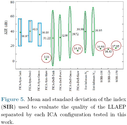
In particular, as indicated by the red circles (and summarized in table 2), independently on the approach, the combination given by FICA-Skew gave the smallest SIR values (3.01 ± 0.00 for the symmetric approach and 14.31 ± 0.00 for the deflation approach), followed by SOBI-124 (16.43 ± 0.00), SOBI-100 (16.90 ± 0.00) and SOBI-150 (17.85 ± 0.00). Regarding the other configurations, the largest mean SIR values (with the smaller standard deviations) were produced by FICA-Sym-Pow3 (40.30 ± 13.22), FICA-Sym-Tanh (38.87 ± 17.24), FICA-Sym-Gauss (36.03 ± 14.15). Conversely, the largest mean SIR values (with the larger standard deviations) were produced by FICA-Defl-Tanh (31.22 ± 34.32), FICA-Defl-Gauss (39.72 ± 30.99), Ext-Infomax-N-1 (39.95 ± 29.42), FICA-Defl-Pow3 (32.09 ± 26.95), and Ext-Infomax-N1 (39.98 ± 24.11).
Finally, on the matter of the computational time required by each ICA configuration, it was found that, as expected, independently on the parameters used, FastICA required the least mean time to estimate the components. In fact, as presented in table 2, it can be seen that the combinations given by FICA-Sym-Skew (0.81 ± 0.16) and FICA-Defl-Skew (0.92 ± 0.06) took in average less than 1 s to estimate the ICs, while FICA-Sym-Tanh (1.82 ± 0.76), FICA-Sym-Gauss (1.70 ± 0.35), FICA-Defl-Tanh (1.88 ± 0.25), FICA-Defl-Pow3 (1.74 ± 0.24), and FICA-Defl-Gauss (1.89 ± 0.71) took a mean time between 1 and 2 s and FICA-Sym-Pow3 (2.12 ± 0.34) took more than 2 s.
Regarding the other ICA implementations tested in this work, only the one given by SOBI-100 (2.90 ± 0.36) required a mean time similar to the time used by FastICA. Conversely, as seen in table 2, the mean time required by the remaining configurations of SOBI and Ext-Infomax were considerably larger, especially for the Ext-Infomax implementation, whose minimum separation time was larger than 40 times the maximum time required by FastICA.
DISCUSSION AND CONCLUSIONS
This work presented a study to identify a suitable ICA implementation/configuration for recovering LLAEPs from simulated EEG/ERP data. It was performed by using three indexes that quantified the global separation accuracy, the LLAEP separation accuracy, and the computational time required by a total of thirteen ICA configurations to estimate the ICs.
According to our results, the combination given by FICA-Sym-Pow3 overcame the performance of the other ICA configurations in both, the global and the LLAEP separation. It was clearly observed on the recovered ICs that, up to the permutation and scaling ambiguities, they remained highly similar to the simulated signals. Such observations were quantitatively confirmed by the separation indexes, which gave the smallest mean Am value and the largest mean SIR value. Also, as indicated by the smaller standard deviations of such indexes, it was evident that FICA-Sym-Pow3 provides a stable separation that, in consequence, makes it possible for this particular configuration of ICA to achieve a robust and quite fast separation (2.1 ± 0.3 s), at least for the component corresponding to LLAEP.
The superior performance of FICA-Sym-Pow3 over other configurations of the same ICA implementation can be explained by the use of Pow3 as the contrast function G, which is recommended to recover sources with "spiky" distributions [26] like the LLAEP one. Thus, by recalling that the separation performance of FastICA is highly dependent on the contrast function used when estimating non-Gaussianity, it was expected to find performance variations among FICA configurations, but never in such a degree that, among the entire set of configurations and implementations tested in this work, they would point at FICASym-Pow3 as the best separation option and at FICA-Defl-Skew as the worst one.
Regarding the time required to estimate the ICs, a general advantage of FastICA is that it does not require as much time to achieve a separation as SOBI and Ext-Infomax. This characteristic is partially achieved by randomly initializing W, which aims to set the optimization process close to the minimum of the contrast function. This strategy helps the algorithm converge faster, but it also makes the method highly dependent on its initialization, and thus, creates the risk for it to converge to a local minimum rather to the global minimum. As a result, the ICs estimated by FastICA from the same dataset might be very different among calculations, which reduce their stability. In our study, this lack of stability was especially evident in the SIR values of the FastICA configurations based on the deflation approach (with the exception of the FICA-Defl-Skew combination), where the standard deviation of the SIR values were close to their average values. This behavior could be produced by the errors accumulated during the successive calculations in the deflation stages, which in consequence turn such combinations into an inappropriate choice for the LLAEP recovery [27].
Regarding Ext-Infomax and SOBI, their configurations presented Am indexes similar to FastICA and their variations remained close to zero. This means that, on the overall separation performance, both algorithms are stable implementations of ICA. However, although Ext-Infomax also managed to achieve a good separation of the LLAEP (according to the SIR values), due to the low learning rate required by its neural network to achieve convergence [28], it took plenty of time to do so (more than one minute to look for a sub-Gaussian IC and more than two and a half minutes on its free configuration). In addition, it produced large variations on the SIR index, which means that Ext-Infomax is more likely to perform unstable LLAEP separations in both configurations (Ext-Infomax-N1 and Ext-Infomax-N-1). SOBI, on the other hand, took less time than Ext-Infomax to separate the ICs (between 2 and 30 s depending on the number of time-lags), but generated very low quality separations of LLAEP, which can be attributed to the wrong selection of that parameter. This means that, for the purpose of recovering the LLAEP from EEG/ERP signals, SOBI is an unsuitable implementation, especially for long-time recordings.
Results so far have been promising and appointed the combination given by FICA-Sym-Pow3 reliable and fast alternative to recover LLAEPs from synthetic EEG/ERP data. Future work will expand this study to include real EEG data (with a synthetic LLAEP) and test these ICA implementations under less restricted conditions.
References
1. Neurophysiology ASC. "Guideline 9A: guidelines on evoked potentials," Am. J. Electroneurodiagnostic Technol., vol. 46, no. 3, pp. 240-53, 2006. [ Links ]
2. C.C. Duncan, R.J. Barry, J.F. Connolly, C. Fischer, P.T. Michie, R. Näätänen, et al., "Event-related potentials in clinical research: guidelines for eliciting, recording, and quantifying mismatch negativity, P300, and N400," Clin Neurophysiol., vol. 120, no. 11, pp. 1883-908, 2009. [ Links ]
3. C.P. Zuluaga, R.C. Acevedo, "Estimación de potenciales evocados auditivos del tronco cerebral mediante descomposición modal empírica," Rev. Mex. Ing. Biomed. , vol. 2, no. 3, pp. 25-30, 2008. [ Links ]
4. N. Castañeda-Villa, C.J. James, "Independent Component Analysis for Auditory Evoked Potentials and Cochlear Implant Artifact Estimation," IEEE Trans Biomed Eng., vol. 58, no. 2, pp. 348-54, 2011. [ Links ]
5. A. Delorme, T. Sejnowski, S. Makeig, "Enhanced detection of artifacts in EEG data using higher-order statistics and independent component analysis," Neuroimage, vol. 34, no. 4, pp. 1443-9, 2007. [ Links ]
6. A.C. Fisher, W. El-Deredy, R.P. Hagan, M.C. Brown, P.J.G. Lisboa, "Removal of eye movement artefacts from single channel recordings of retinal evoked potentials using synchronous dynamical embedding and independent component analysis," Med Biol Eng Comput, vol. 45, no. 1, pp. 69-77, 2007. [ Links ]
7. D.M. Groppe, S. Makeig, M. Kutas, S. Diego, "Independent Component Analysis of Event-Related Potentials," Cogn Sci Online, pp. 1-44, 2008. [ Links ]
8. C. James, C. Hesse, "Independent component analysis for biomedical signals," Physiol Meas, vol. 26, no. 1, pp. R15-39, 2005. [ Links ]
9. C.A. Joyce, I.F. Gorodnitsky, M. Kutas, "Automatic removal of eye movement and blink artifacts from EEG data using blind component separation," Psychophysiology, vol. 41, pp. 1-13, 2004. [ Links ]
10. M. Klemm, J. Haueisen, G. Ivanova, "Independent component analysis: comparison of algorithms for the investigation of surface electrical brain activity," Med Biol Eng Comput., vol. 47, no. 4, pp. 413-23, 2009. [ Links ]
11. A. Craig, P. Boord, D. Craig, "Using independent component analysis to remove artifact from electroencephalographic measured during stuttered speech," Med Biol Eng Comput. , vol. 42, pp. 627-33, 2002. [ Links ]
12. A. Hyvärinen, E. Oja, "Independent component analysis: algorithms and applications," Neural Networks, vol. 13, no. 4-5, pp. 411-30, 2000. [ Links ]
13. G.R. Naik, D.K.Kumar, "An Overview of Independent Component Analysis and Its Applications," Informatica, vol. 35, pp. 63-81, 2011. [ Links ]
14. R.J. Korhonen, J.C. Hernandez-Pavon, J. Metsomaa, H. Máki, R.J. Ilmoniemi, J. Sarvas, "Removal of large muscle artifacts from transcranial magnetic stimulation-evoked EEG by independent component analysis," Med Biol Eng Comput. vol. 49, no. 4, pp. 397-407, 2011. [ Links ]
15. D. Iyer, G. Zouridakis, "Estimation of Brain Responses Based on Independent Component analysis and wavelet denoising," Technical Report Number UH-CS-05-01, Biomedical Imaging Lab Department of Computer Science University of Houston, pp. 1-12, 2005. [ Links ]
16. N. Yeung, R. Bogacz, C.B. Holroyd, S. Nieuwenhuis, J.D. Cohen, "Theta phase resetting and the error-related negativity," Psychophysiology, vol. 44, no. 1, 39-49, 2007. [ Links ]
17. P.E. McSharry, G.D. Clifford, L. Tarassenko, L.A. Smith, "A Dynamical model for Generating Synthetic Electrocardiogram Signals," IEEE Trans Biomed Eng. , vol. 50, no. 3, pp. 289-94, 2003. [ Links ]
18. A. Hyvärinen, E. Oja, "A Fast Fixed-Point Algorithm for Independent Componet Analysis," Neural Comput., vol. 9, pp. 1483-942, 1997. [ Links ]
19. A.J. Bell, T.J. Sejnowski, "An information-maximisation approach to blind separation and blind deconvolution," Neural Computation, vol. 7, no. 6, pp. 1129-1159, 1995. [ Links ]
20. A. Belouchrani, K. Abedmeraim, "A Blind Source Separation Technique Using Second-Order Statistics," IEEE Trans Signal Process, vol. 45, no. 2, pp. 434-44, 1997. [ Links ]
21. T-W. Lee, M. Girolami, T.J. Sejnowski, "Independent Component Analysis Using an Extended Infomax Algorithm for Mixed Subgaussian and Supergaussian Sources," Neural Comput., vol. 11, no. 2, pp. 417-41, 1999. [ Links ]
22. W. Zhou, D. Chelidze, "Blind source separation based vibration mode identification," Mech Syst Signal Process., vol. 21, no. 8, pp. 3072-87, 2007. [ Links ]
23. T. Lee, T.J. Sejnowski, "Independent Component Analysis for Mixed Sub- Gaussian and Super- Gaussian Sources," Jt Symp Neural Comput. , vol. 4, pp. 132-9, 1997. [ Links ]
24. A. Cichocki, S. Amari, "Robust Techniques for BSS and ICA with Noisy Data," Adaptive Blind Signal and Image Processing, pp. 307-8, 2002. [ Links ]
25. G. Gómez-Herrero, A. Gotchev, K. Egiazarian, "Distortion Measures for Sparse Signals," Int Conf Comput Syst Technol - CompSysTech' 2005, vol. 2, pp. 1-6, 2005. [ Links ]
26. A. Delorme, S. Makeig, an open source toolbox "EEGLAB: for analysis of single-trial EEG dynamics including independent component analysis," J Neurosci Methods, vol. 134, no. 1, pp. 9-21, 2004. [ Links ]
27. E. Ollila, "The Deflation-Based FastICA Estimator: Statistical," IEEE Trans Signal Process, vol. 58, no. 3, pp. 1527-41, 2010. [ Links ]
28. F. Raimondo, J.E. Kamienkowski, M. Sigman, D. Fernandez Slezak, "CUDAICA: GPU optimization of Infomax-ICA EEG analysis," Comput Intell Neurosci, vol. 2012, 206972, 2012. [ Links ]

