Artículos de investigación original

 

Analysis of the Inverse Electroencephalographic Problem for Volumetric Dipolar Sources Using a Simplification

 

Análisis del Problema Inverso Electroencefalográfico para Fuentes Dipolares Volumétricas por Medio de una Simplificación

 

J.J. Oliveros-Oliveros* M.M. Morín-Castillo** F.A. Aquino-Camacho* A. Fraguela-Collar*

 

* Facultad de Ciencias Físico Matemáticas, Benemérita Universidad Autónoma de Puebla.

^** Facultad de Ciencias de la Electrónica, Benemérita Universidad Autónoma de Puebla.

 

Correspondencia:
José Jacobo Oliveros Oliveros
Edificio 111A/201F, 18 Sur y
Ave. San Claudio, Col. Jardines
de San Manuel, Puebla, Pue.
México, CP 72570.
Tel. (01 222) 22 9 55 00 ext.
2119, 2178.
Correo electrónico: oliveros@fcfm.buap.mx

 

Fecha de recepción: 19 de diciembre de 2013
Fecha de aceptación: 22 de mayo de 2014

 

ABSTRACT

Objective: To analyze the parameter identification problem for volumetric dipolar sources in the brain from measurement of the EEG on the scalp using a simplification which reduces the multilayer conductive medium problem to one homogeneous medium problem with a null Neumann boundary condition. Methodology: The minimum squares technique is used for parameter identification of the dipolar sources. The simple case in which the head is modelled by concentric circles is developed. This case was chosen because we were able to obtain the solution of the forward problem in exact form and for the simplicity of the exposition. Results: The parameter of the dipolar sources can be identified from the EEG on the scalp using the simplification. For the theoretical analysis the results developed for one homogeneous region are used. The numerical implementation is simpler than the multilayer case and the numerical computation requires minor computational cost. Conclusion: The feasibility for solving the parameter identification problem using the simplification is shown. These results can be extended to the case of concentric spheres and complex geometries but the solution cannot be found in exact form.

Keywords: inverse electroencephalographic problem, volumetric dipolar sources, Green function.

 

RESUMEN

Objetivo: Analizar el problema de identificación de los parámetros para fuentes dipolares volumétricas en el cerebro a partir de la medición del EEG en el cuero cabelludo mediante una simplificación que reduce el problema de un medio conductor de múltiples capas a un problema en un medio homogéneo con una condición de Neumann nula en su frontera. Metodología: Se utiliza la técnica de mínimos cuadrados para identificar los parámetros de las fuentes dipolares. Se desarrolla el caso simple en el que la cabeza está modelada por círculos concéntricos debido a que la solución del problema directo se puede calcular en forma exacta y por la sencillez de la exposición. Resultados: Se identifican los parámetros de la fuente dipolar a partir del EEG sobre el cuero cabelludo usando la simplificación. Para el análisis teórico se utilizan los resultados desarrollados para una región homogénea. La implementación numérica es más simple y el cálculo numérico requiere menor costo computacional. Conclusión: Se muestra la factibilidad para resolver el problema de identificar los parámetros de una fuente dipolar por medio de la simplificación. Los resultados pueden ser extendidos al caso de esferas concéntricas y al de geometrías complejas pero la solución del problema directo no puede hallarse en forma exacta.

Palabras clave: problema inverso electroencefalográfico, fuentes dipolares volumétricas, función de Green.

 

INTRODUCTION

Different non-invasive techniques for brain scans have been developed using mathematical models. These include positron emission tomography, magnetic resonance imaging and electroencephalography. This final technique is the present study focus. Electroencephalography is the best known among the non-invasive brain investigation methods. It is based on the use of scalp located electrodes to record brain electrical activity. This recording is known as the Electroencephalogram (EEG). The electrical activity is generated by the bioelectrical activities of large neuron populations working synchronously [1, 2]. The EEG technique allows us to detect anomalies in the brain (damage, malfunction, etc.) which have traditionally been done by different diagnostic techniques. The problem is studied through a boundary value problem, which is obtained using a model that describes the head as a conductive layer medium. This model allows finding relationships between the characteristics of the bioelectrical activity and the EEG.

This paper presents the analysis of the inverse problem for dipolar sources in the brain from measurement of the EEG on the scalp. This analysis uses a simplification in which the original problem is reduced to a problem in a homogeneous region with a null Neumann condition along with a "measurement" (which is obtained from the EEG) on the boundary of the mentioned homogeneous region (Cauchy data). For the analysis and the simplicity of the exposition, the head is modelled for two concentric circles. This allows the forward problem calculation in exact form. Two auxiliary problems are solved in exact form too. For that, the Green function for the Poisson equation with a null Neumann boundary condition in a circular homogeneous region and the circular harmonics are used.

 

MATHEMATICAL MODEL

We will suppose that the human head, considered as conductive medium, is divided in two disjoint zones as illustrated in Fig. 1. Where Ω = U Ω₂ represents the head, Ω_i the brain, Ω₂ the rest of the head, σ_i and σ₂ are the constant conductivities of Ω_i and Ω₂, S₁ represents the cerebral cortex and S₂ the scalp.

The study of the Inverse Electroencephalogra phic Problem (IEP) can be made through the following boundary value problem [1, 3, 4, 5]:

where f is called the source, u_i = u|_Ωi, i = 1,2, u represents the electrical potential in Ω, and , i = 1,2 denote the normal derivative of u_i on S_j regarding the normal unitary vector n_j, j = 1,2. The boundary conditions (3)-(4) are called the transmission and the condition (5) is obtained when we consider the conductivity of air equal zero. We will call this problem the Electroencephalographic Boundary Problem (EBP).

From the Green formulas the following compatibility condition is deduced

In the next section, we will study the identification problem of the function f given in (1) using the boundary value problem (1)-(5) and the additional boundary condition:

 

SIMPLIFICATION OF THE INVERSE EEG PROBLEM TO ONE IN A HOMOGENEOUS REGION

The simplification is achieved through the following steps:

1. We can find the harmonic function u₂ through the Cauchy data u₂ = V and = 0 on the boundary S₂.

2. Making ψ = we solve the problem to find a harmonic function in Ω₁ which satisfies the boundary condition = ψ. We take the solution which is orthogonal to the constants in order to have uniqueness of the solution. The compatibility condition of ψ is given by ∫s₁ ψ(s)ds = 0, which is deduced from the Green formulas.

3. Now, we consider the following inverse source problem: Find the source f that satisfies the problem

using the additional data on S₁ :

where ø = u₂|_S1.

From this we see that the IEP can be solved through the previous inverse problem. The problem (7-8) is called the Inverse Electroencephalographic Simplified Problem (IESP).

The development of this section is valid for general regions with sufficiently smooth boundaries.

 

STATEMENT OF THE INVERSE PROBLEM FOR DIPOLAR SOURCES

In this paper we are interested in the case where the source is an epileptic focus. In general, the current distributions describing sources of neural activity are quite intricate. A common simplifying assumption is to consider a current dipole as a source. This model, which is known as the equivalent current dipole, has been shown to accurately depict sources not too deep inside the brain [6] and to permit the associated estimation and accuracy analysis to be carried out fairly simply. More complicated shapes may be approximated by multiple dipoles or multipolar expansions. For simplicity, in this work, we consider only a single dipole of current density. In this case, the source f can be represented in the form [1]

where p represents the dipolar moment (that determines the intensity and orientation of the dipole) and δ(x — α) is the Dirac delta concentrated in a. In this case we have uniqueness of solution for the inverse problem if the measurement V is known on the whole scalp.

We suppose that measurement V is known.

With the ideas presented in the previous section, we can recover the parameters of the dipole source, namely, the dipole moment p and its location a, through the minimum squares functional

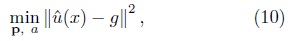
where û is the solution of the problem (7) and g is given by (8) and, of course, û is given in terms of the source f and g in terms of V. Some iterative method must be used for the minimization process. In section 6, we apply the function fmincon of MATLAB which uses a Newton type method.

The solution of the problem (7) when f is given by (9) is [5]

where G(x, y) is the Green function of the problem (7). The main inconvenience with the Green function technique is due to the difficulty of finding it when the geometry is not simple.

In the case of general smooth boundaries, in which we can't use the Green function technique, the ideas presented in this work can be developed using numerical methods (as the boundary element and finite element) since the solution of the problems presented in the last section must be found numerically. This is not considered in this work.

 

DEVELOPING THE IDEAS IN THE SIMPLE CASE OF CONCENTRIC CIRCLES

In order to validate the ideas presented in section 3, the forward problem must be solved. For simplicity of the exposition we consider the case in which the human head is modelled through two concentric circles. We chose this case due to the solution of the forward problem can be calculated in exact form without using numerical methods which is important since we can build synthetic examples for validating the reduction to one problem defined in a homogeneous region. The results of this section can be extended to the case of concentric spheres but in this case we must calculate numerically some integral associated with the Fourier coefficient of the measurement (solution of the forward problem). The case of complex geometries can be solved with the method presented in this work, but it is necessary to use numerical methods for solving the forward and the inverse problems. But even in this case, the proposed method gives advantages because we need fewer calculations. According to the ideas presented in this work the inverse problem is reduced to one in a circular homogeneous region and for this case we will use the Green function technique.

 

Green's function for the problem (7)

The Green function G(x, y) defined in Ω₁ x Ω₁ of the problem (7) satisfies the boundary value problem:

For the case when Ω₁ corresponds to circle of radius R = R₁, the Green function is given by

where is the complex conjugate of y [5].

The Green function for the spherical case can be found in [7, 8].

 

Solution of the forward problem

In order to find the solution of the forward problem, we consider the following auxiliary boundary value problem

where g(x) = û(x) = [∇yG(x, y)]|_y=α x ∈ S₁. The solution of the problem (14)-(18) is unique in the orthogonal space to the constants [9].

The solution to the problem (1)-(5) is given

Now, we calculate the solution of the problem (13)-(17) which can be expressed in the form:

From (16) and (17) we get

where ,i = 1,2 are the Fourier coefficients g and g(θ) = of cos kθ + sin kθ.

From (21) and (22) we find

Now, using the condition (18) we get

From (23) and (24)

Substituting (25)-(28) in (21), we find

The coeficients (25)-(30) give the solution to the problem (14)-(18) and the measurment is given by V = cos (kθ) + sin (kθ) where

Now we calculate the Fourier expansion of the function g = [∇yG(x, y)]|_y=α.

As a first step we must calculate ∇yG(x, y). After some calculations we get

Let p = (p₁,p₂). Then

Taking into account that the solution is orthogonal to the constants, the terms and were neglected. We denote x₁ = R₁ cos(θ), x₂ = R₁ sin(θ), y₁= r cos(θy) and y₂ = r sin(θy). After substituting this in (34) we obtain

Now, we calculate the Fourier coefficients of g.

It is necessary to calculate the following integrals

For that we need the following integrals

It can be seen that

where we use the notation x = R₁e^iθ y = r₀e^iθy. In effect,

and taking into account that dx = ixdθ , then

where now the differential is complex. From this

We define Φ(y) = . Note that = where x₀ = y. Since Φ is analytical in Ω₁ we have that

Analogously

Using trigonometric identities we get

from where

and

The restriction of the function w₂ to S₂ gives the solution of the forward problem.

 

Solution of the inverse problem

For solving the inverse problem we suppose that the measurement is given by V = cos(kθ) + sin(kθ). The first step consists of finding the function u₂ (solution of the Cauchy problem in Ω₂ ) from V. After some calculation we find

The second step consists of finding the harmonic function ū in Ω_1, orthogonal to the constants, that satisfies the Neumann condition = ψ = . This function is given by

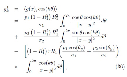
From this, the "measurement" g on S₁ is given by

Note that in (44) the Fourier coefficients of g are in terms of and . On the other hand, these Fourier coefficients are given in terms of the parameters of the dipolar source p and a. The next step consists of determining, from the measurement V, the parameters of the dipole p and a through the least squares functional (10). In the following, we suppose thatandare known. We have to minimize the functional

where and are the approximations of the Fourier coefficients obtained using (44) when the Fourier coefficients of V have errors and N is chosen appropriately such as [10] and [11] (for two and three dimensions, respectively) for the ill-posedness of the problem due to the numerical instability.

When the measurement is given at a finite number of points on the scalp, we can obtain the measurement on the whole scalp using a regularized interpolation method such as presented in [12].

Simple geometries for the analysis of the inverse electroencephalographic problem have been used. For the case of a dipolar source in [13] a method for finding its location is presented which is based on rational approximations in the complex plane. In [14] an algorithm for finding a dipole from Cauchy data is given considering a spherical model for the head.

 

NUMERICAL EXAMPLES

In this section we present synthetic examples in order to show the ideas presented in this work. We consider that R₁ = 1.2, R₂ = 2, σ₁ =3 and σ₂ = 1. We take as the parameters of the dipolar source p = (p₁,p₂) = (0.5,0.5) and (r₀,θ_y) = (0.7, ^π/3) (polar coordinates).

Using (31), (32), (40) and (41) we calculate the corresponding measurement V. In order to simulate the inherent error of the measurement V^δ due to the equipment, a random error to the Fourier coefficients of V such that || V - V^δ|| _L2S2 < δ it is included. In this case we have the following approximation to the function g:

We made programs in MATLAB for determining the parameters of the dipolar source taking as input data the values given in (46) and using the fmincon function which use a Newton type method. In Table 1, the results obtained are presented. For the election of the initial point of the iterative method we can use additional information about the problem (a priori information). We take δ= 0. 1 and N = 10.

The ill-posedness of the problem due to the numerical instability must be taken into account for obtaining a stable solution.

The ideas presented in this work can be used for more realistic geometries of the head along with numerical methods such as finite element method. In [15] numerical methods for dipoles identification are proposed, namely, the finite element method and the boundary element method.

 

CONCLUSIONS

The problem of determining the epileptic focus from EEG on the scalp has been studied through a model that consider the head as a multilayer conductive medium as well as the quasi static approximation of Maxwell equations which address one boundary value problem that allows establishing relationships between epileptic focus and the EEG. The multilayer model can be reduced to one problem in a homogeneous region with a null Neumann condition. From this, the problem of determining the parameters of the dipolar source is analysed in the homogeneous region mentioned above. This is conceptually and numerically more simple than multilayer case. The proposed method is validated numerically through synthetic examples for the case of concentric circles. This simple case was chosen because we were able to obtain the solution of the forward problem in exact form and this fact is used for validating the proposed method. In a similar way, these examples can be developed for the case of multilayer spherical geometry which is commonly used for the study of this problem. Even more, this can be used for more realistic geometries of the head along with numerical methods such as the finite element method. For the case of a finite number of points on the scalp in which the measurement is given, we must apply stable interpolation methods for obtaining the measurement on the whole scalp for the uniqueness of the solution of the inverse problem. However this is not considered in this work.

 

REFERENCES

1. Sarvas J. Basic Mathematical and Electromagnetic Concepts of the Biomagnetic Inverse Problem. Phys. Med. Biol., 1987; 32(1): 11-22.         [ Links ]

2. Nuñez PL. Electric Field of the Brain. Oxford Univ. Press, New York (USA), 1981.         [ Links ]

3. Fraguela A, Oliveros J and Morín M. Mathematical Models in EEG inverse, in: Jiménez Pozo MA, Bustamante J, Djorjevich S, Editors, Topics in the Theory of Approximation II (in Spanish). Scientific Texts, Autonomous University of Puebla (México), 2007; 73-95.         [ Links ]

4. Grave R, González S and Gómez CM. The biophysical foundations of the localization of encephalogram generators in the brain. The application of a distribution-type model to the localization of epileptic foci (in spanish). Rev. Neurol. , 2004; 39: 748-756.         [ Links ]

5. Fraguela A, Morín M. and Oliveros J. Inverse problem statement for locating the parameters of a neural current dipolar source (in spanish). Communications of Mexican Mathematical Society , 1999; 25: 41-55.         [ Links ]

6. Muravchik CH and Nehorai A. EEG/MEG Error bounds for a static dipole source with a realistic head model. IEEE Transactions on Signal Processing , 2001; 49(3): 470-484.         [ Links ]

7. Sobolev SL. Partial Differential Equations of Mathematical Physics (in spanish). Addison-Wesley Publishing Company, Inc. (Moscú), 1964.         [ Links ]

8. Morín M, Oliveros J, Conde J, Fraguela A, Gutierrez EM and Flores E. Simplification of the inverse electroencephalographic problem to one homogeneous region with null Neumann (in Spanish). Revista Mexicana de Ingeniería Biomédica, 2013; 34(1): 41-51.         [ Links ]

9. Fraguela A, Oliveros J and Grebennikov A. Operational statement and analysis of the inverse electroencephalographic problem. Revista Mexicana de Física, 2001; 47(2):162-174.         [ Links ]

10. Fraguela A, Morín M. and Oliveros J. Inverse electroencephalography for volumetric sources. Mathematics and Computers in Simulation, 2008; 78: 481-492.         [ Links ]

11. Oliveros J, Morín M, Conde J and Fraguela A. A regularization strategy for the inverse problem of identification of bioelectrical sources for the case of concentric spheres. Far East Journal of Applied Mathematics, 2013; 77: 1-20.         [ Links ]

12. Bustamante J, Castillo R and Fraguela A. A regularization method for polynomial approximation of functions from their approximate values at nodes. Journal of Numerical Mathematics, 2009; 17(2): 97-118.         [ Links ]

13. Clerc M, Leblond J, Marmorat JP and Papadopoulo T. Source localization using rational approximation on plane sections. Inverse Problems, 2012; 28(5): 055018 (24pp).         [ Links ]

14. Tsitsas N and Martin P. Finding a source inside a sphere. Inverse Problems, 2012; 28: 015003 (11pp).         [ Links ]

15. Pursiainen S, Sorrentino A, Campi C and Piana M. Forward simulation and inverse dipole localization with the lowest order Raviart-Thomas elements for electroencephalography. Inverse Problems, 2011; 27: 045003 (17pp).         [ Links ]