nova página do texto(beta)
 Inglês (pdf)
 Artigo em XML
 Referências do artigo
 Enviar este artigo por email
 Citado por SciELO
  Similares em
SciELO
Similares em
SciELO 
 Permalink
INTRODUCTION
Environmental flows are defined as hydrologic regimes that are requi red to sustain ecosystem health and functions in rivers, wetlands or coastal regions, where there are competing and diverse water uses and flows are regulated. The concept was developed to assure that aquatic ecosystems are left with the necessary water quantity and quality to maintain their biotic structure (Dyson et al., 2008). Numerous terms define the same concept: environmental flow (39%), minimum flow (38%), in-stream flow requirement (37%), ecological reserve (23%) and other terms (21%) (Moore, 2004). Different methodologies have been developed to establish the environmental flows in rivers (Dyson et al., 2008). E.g., Tharme (2003) registered a minimum of 207 methodo logies (29% hydrological, 28% habitat simulation, 17% combination, 11% hydraulic, 8% holistic and 7% others).
The Instream Flow Incremental Methodology (IFIM) is a theoretical framework to evaluate the ecological flow requirement of rivers (Bovee et al., 1998; Stalnaker et al., 1995; Waddle, 2001). It provides an or ganizational structure for the evaluation and formulation of water ma nagement alternatives that respond to the interests of different water uses (Stalnaker et al., 1995). The PHABSIM (Physical Habitat Simu lation Model) simulation model (Milhous et al., 1989; Waddle, 2001) is used to calculate the available habitat useful in a river segment for different species in different flows. PHABSIM employs a structure defi ned by stream morphology, hydraulic parameters and habitat suitability criteria (Bovee et al., 1998; Milhous, 2007; Stalnaker et al., 1995). The IFIM-PHABSIM methodology is based on the concept of Weighted Usea ble Area (WUA), i.e., the wetted stream area is weighted by empirically derived from fish species’ microhabitat preferences (Stalnaker et al., 1995). WUA-Q curves provide a measure of the available habitat as a function of stream flow (Waddle, 2001).
The Mexican standard NMX-AA-159-SCFI-2012 (DOF, 2012) esta blishes the procedure for evaluating ecological flows in basins. This re gulation refers to hydrological methodologies as the simplest approach to get results in the short run; as illustrated by the case studies of the River Valley in San Luis Potosi (Santacruz de León & Aguilar-Robledo, 2009) and the Acaponeta River in Nayarit, Mexico (De la Lanza et al., 2012). The habitat simulation methodology, on the other hand, requires more detailed information in terms of hydrological, hydraulic and biolo gical data (this IFIM-PHABSIM approach has recently gained significant importance in Mexico). Finally, holistic methods are recommended for basins with highly varying flow regimes and whose characteristics have been significantly altered. They require a greater amount of information and resources (hydrological, hydraulic, biological, ecological, economic, and social). The aim of this paper is to propose an environmental flow requirement in a fluvial segment of the Duero River Basin (DRB) through the habitat simulation method, using five fish species as indicator spe cies.
The DRB. This basin comprises an area of 2198 km2 (CONAGUA, 2009) and is located in northwest Michoacan state, Mexico (Fig. 1). The Duero River has its source at the springs in the town of Carapan, and flows through the Cañada de los Once Pueblos. Its main tributaries are the Celio River from the south (south of Jacona) and the Tlazazalca River from the northeast (northeast of Tangancicuaro). The flow in Tlazazalca River is regulated by the Urepetiro dam for flood control (Zavala-López, 2011). Further downstream along Duero River, Irrigation District 061 consists of 18,000 hectares of agricultural land and four irrigation mo dules: I) Urepetiro-Verduzco (20%), II) Principal Chaparaco (30%), III) Río Nuevo (24%), and IV) Peñitas-Estanzuela (26%) (CONAGUA-IPN, 2009). Figure 1 shows that the study area is located at the mouth of the basin. It consists of a river segment of 11.6 km length between the town of San Simon-La Estanzuela and the Camucuato Bridge.

The DRB contains a wide variety of natural resources, i.e., rivers, springs and aquifers, as well as oak and pine forests. The aquatic bio diversity consists of numerous fish species and macroinvertebrates. The hydraulic infrastructure consists of reservoirs and dams, agricultu ral areas, channels, wells, sewage treatment plants and drinking water systems (Velázquez et al., 2005, 2010). The catchments of the DRB face environmental problems such as deforestation, land use change, and the proliferation of invasive species. Other current issues include increasing urbanization, lack of specific sites for solid waste disposal, wastewater discharge into the rivers (CONAGUA-IPN, 2009; Velázquez et al., 2005).
Moncayo-Estrada et al. (2014) evaluated the index of biological in tegrity (IBI) for the year 2009 in the Duero River and compared it with indexes obtained in 1986 and 1991. The comparison revealed that the sampling sites of Camecuaro Lake and Camucuato Bridge changed their status from good to fair and poor, respectively. Further, El Capulin, Zamora, La Estanzuela and San Cristobal “A” deteriorated from fair to poor. The environmental degradation that is responsible for this dete rioration in biological integrity is attributed to excessive water use and wastewater discharges.
Fish communities. Fish communities are the most common biological group used to assess the environmental quality of freshwater ecosys tems in Mexico (Mathuriau et al., 2011). The NMX-AA-159-SCFI-2012 (DOF, 2012) also highlights that the experience in selecting target spe cies is more developed for fish (at a national and international level) than for any other animal group. In the DRB, a variety of fish species is to be found. E.g., Ledesma-Ayala (1987) collected 1393 specimens belon ging to 16 different species. In this study, the classification of tolerance towards environmental degradation (tolerant, medium-tolerant, sensi tive) was the main criterion for the selection of species. Therefore, the ichthyic fauna in the DRB is represented by three families: Atherinidop sidae (species: Menidia jordani (Woolman, 1894)), Cyprinidae (species: Algansea tincella (Valenciennes, 1844) and Aztecula sallaei (Günther, 1868); and Goodeidae (species: Goodea atripinnis (Jordan, 1880) and Alloophorus robustus (Bean, 1892)). According to Ibáñez et al. (2008) and Miller et al. (2009)Menidia jordani (previously Chirostoma jordani (Woolman, 1894)) is a fish that inhabits clear or turbid waters in rivers and channels with depths of 1 m. Algansea tincella is found from small streams to large lakes. Spawning occurs from May to July (Barbour & Miller, 1978; Miller et al., 2009). Algansea tincella lives in water bodies with rocky bottoms to finer sediments (Ledesma-Ayala, 1987). Goodea atripinnis is a prolific fish; juveniles appear at the end of January and mid-July, which indicates a prolonged reproductive season (Miller et al., 2009). López-Eslava (1988) concluded that G. atripinnis reproduces between April and May, whereas Barragán & Magallón (1994) indica te that the reproduction period extends from April to September. The habitat includes clear or turbid waters in streams and it is commonly found in shallow areas (0.5 to 1.7 m). Alloophorus robustus is typically found in rivers with clay and gravel beds; the depths range from 1 to 2 m. The juvenile stage occurs in mid-May and June (Miller et al., 2009). The reproductive period extends from April to June (Mendoza, 1962). However, according to Soto-Galera et al. (1990), females experience a simple reproductive cycle from July to August. Aztecula sallaei (Notro pis sallei (Günther, 1868)) inhabits ponds fed by streams and channels, which generally consist of fine-gravelly substrates in depths that ran ge from 0.5 to 1.3 m in the water column. In streams, the preferred current ranges from moderate to quick and occasionally strong. The spawning period most likely occurs from February to April and possibly extends until May (Miller et al., 2009). Although the reproductive period extends from March to September (Sánchez & Navarrete, 1987), June and July have been registered as the months of greatest reproductive intensity (Navarrete & Sánchez, 1987).
Table 1 summarizes some of the ecological attributes of these five fish species and shows four different evaluations of the species’ tolerance of environmental degradation, over a period of 17 years. According to Lyons et al. (1995I, 2000II), Mercado-Silva et al. (2006III) and Ramírez-Herrejón et al. (2012IV) tolerance was evaluated in the following manner: M. jordani maintains a ‘tolerant’ status (II, III, IV); A. tincella changed from ‘tolerant’ to ‘medium-tolerance’ (I, II, III, IV); A. sallaei’s assessment chan ged from ‘medium-tolerance’ to ‘sensitive’ (II, III); G. atripinnis has main tained a ‘high tolerance’ over time (I, II, III, IV); whereas the A. robustus changed from a ‘medium-tolerance’ to a ‘sensitive’ evaluation in 2012.
Table 1 Ecological attributes of fish species found in the Duero River, Mexico.
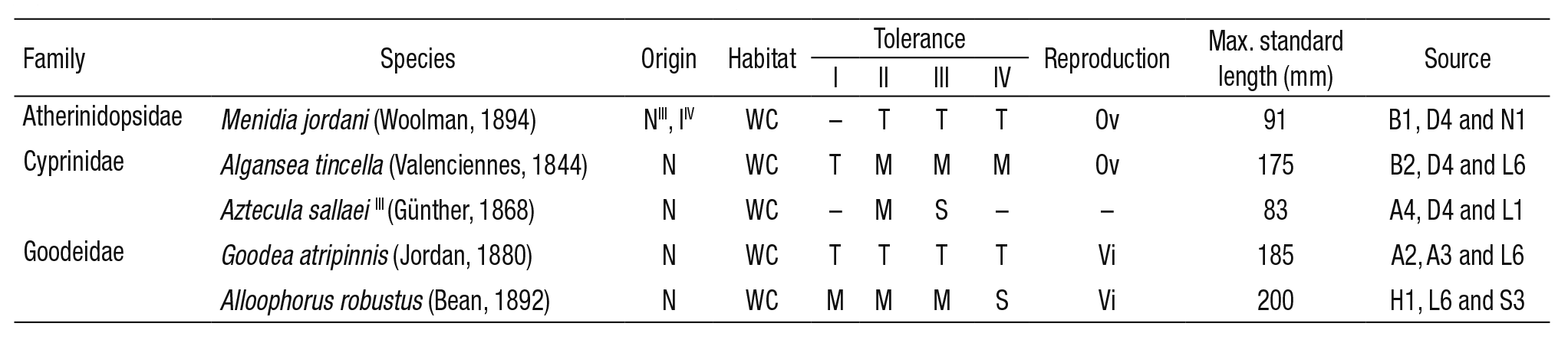
Origin (N: native species, and I: introduced); habitat (WC: water column); tolerance (T: tolerant, M: medium-tolerance and S: intolerant/sensitive); reproductive type (Ov: oviparous and Vi: viviparous); max. standard length in mm. Sources: (B1) Barbour (1973); (D4) Díaz-Pardo et al. (1993); (N1) Navarrete et al. (1996); (B2) Barbour & Miller (1978); (L6) Lyons et al. (1995); (A4) Álvarez & Navarro (1957); (L1) López-López & Vallejo de Aquino (1993); (A2) Álvarez (1963); (A3) Álvarez & Cortes (1962); (H1) Hubbs & Turner (1939); (S3) Soto-Galera et al. (1990). I and II: Lyons et al. (1995, 2000); III: Mercado-Silva et al. (2006); IV: Ramírez-Herrejón et al. (2012).
MATERIALS AND METHODS
The procedure for proposing the environmental flow requirement (EFR) in the lower basin of the Duero River is the Instream Flow Incremental Methodology (IFIM) (Bovee et al., 1998; Stalnaker et al., 1995; Waddle, 2001), which covers the following steps:
Scope of the study. Currently, the Duero River Basin is subject to va rious pressures from the agricultural sector and various stakeholders, in addition to being an ecological habitat. Due to regulatory activity, it is necessary to review the status of the river and to propose an environ mental flow regime that will continue to support the river ecosystem.
Selection of the hydraulic model. PHABSIM quantifies the habitat, defined as the optimum flow that maximizes the area available for each species (Orth & Leonard, 1990). For each flow, the available habitat is calculated by adding the area of each computational cell that comprises the control section to its corresponding composite suitability index, as expressed by Equation (1) (Bovee et al., 1998; Milhous et al., 1989; Moir et al., 2005; Waddle, 2001).
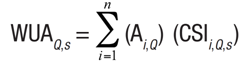 (1)
(1)where WUAQ,s is the weighted usable area for the given discharge (Q) for target species (s), Ai is the area of each computational cell (i), and CSIi,Q,s is the composite suitability of computational cell (i) at discharge (Q) for target species (s). WUA is expressed in units of habitat area, m2 per unitized distance along a stream, 1000 m or 1 km (Waddle, 2001). The CSI is non-dimensional, expressed by Equation (2) (Bovee et al., 1998):
 (2)
(2)where HSI is the habitat suitability indices, according to the velocity (vi), depth (pi) and substrate (si) variables (Waddle, 2001), and expres ses the degree of adaptation of an organism to these variables (0 un suitable to 1 most suitable) (Bovee et al., 1998; Stalnaker et al., 1995).
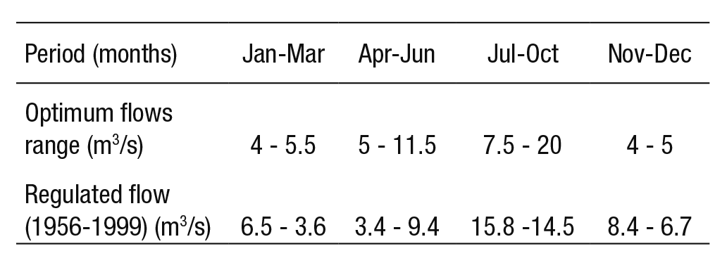
Hydrologic regime (natural and regulated). Daily flow records were obtained from the hydrometric station (12310) (BANDAS, 2006). We identified two periods: The first period extends from 1936 to 1955 and is named the natural flow regime (NFR); the second period from 1956 to 1999 corresponds to the regulated flow regime (RFR). Figure 2 shows the variation in river flow before and after the hydraulic regulation in the indicated periods. The total annual difference between average mon thly flows of the NFR and RFR is less than 10%, whereas the minimum regulated flow regimes (mRFR) show a decrease of 43% relative to the minimum natural flow regimes (mNFR).

The dry season of the NFR curve lasts from January to May, with an average flow of 7.61 to 6.66 m3/s; except in April, when it is 4.92 m3/s. The rainy season is reflected by the increased flows from June (8.47 m3/s) to September (25.79 m3/s). In the mid-1950s, the DRB experien ced flow variations. During the dry season, the RFR curve was reduced by 26% (registering 3.44 m3/s for April); and during the rainy season, the RFR curve increased 18%, with respect to the natural regime.
In dry season, the mNFR curve shows flows of 3.41 and 3.38 m3/s, in March and April respectively. Minimum flow rates during March, April, and May have decreased by 80% with regulation, when compa ring the mRFR and mNFR curves. In sum, Figure 2 shows that the re gulated regime (RFR) now has similar conditions to the natural behavior of the minimum flows (mNFR).
Characterization of the fluvial segment. The slope of the river was defined by tracing a curve every 20 meters in a digital terrain model (DTM) of the area. The measurement sites (transect/cross-section) were identified on the map and in the field; as well as inflows and flow diversions. The model should consider the river reach as a closed system where the continuity equation may be applied (inlet and outlet flows do not vary with time). In addition, the hydrometric station is identified for historical flow records and biological information to gene rate suitability curves.
River cross-sectionals were generated using a digital theodolite (DTW-10) and a flow meter (GPI-1100) to measure the velocity across the water column. We chose the density of points along the cross sec tion where the depth and velocity of the water column was measured according to the regularity or irregularity of the stream bed and the intensity of the flow; i.e., for uniform beds less detail was given on the measurements, whereas for higher velocities greater detail was applied. That way, six transects were measured along the river reach. According to Payne et al. (2004) the total number of transects should be proportional to the complexity of the hydraulic system: 6 to 10 transects for simple reaches and 18 to 20 transects for diverse reaches. The measuring period of the hydraulic variables occurred during February 2011.
Table 2 summarizes the hydraulic characteristics of the six tran sects (Estanz, sr66, sr63, sr62, sr60, siz68) such as depth, velocity, and dominant substrate; length and average slope of the river. The water surface level (WSL), thalweg, and width of free-surface flow (WFS) was determined through bathymetry of the river transects, displaying the output results on a spreadsheet. The riverbed substrate presented a variety of materials, from fine sediments (clays, silts and sands) to pe bbles. According to the standard characterization of substrate values used by PHABSIM (Bovee, 1986), were assigned to the riverbed as a function of the predominant material in the cross section. The type of mesohabitat was identified according to the classification made by Sanz-Ronda et al. (2005). The flow volume in the control sections was obtained by applying the central cell division method. The average flow measured in the cross sections was 3.02 m3/s.
Table 2 Physical characteristics of the study reach, composed of six transects, for use in the PHABSIM model.
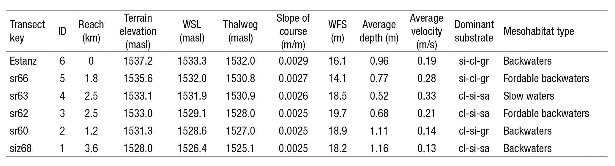
Cross section (first column); (ID) transect number; length; terrain elevation of the river bank; (WSL) elevation of water surface level of the river; (thalweg) elevation at maximum depth of the cross section; slope of the water length; (WFS) width of free-water surface of the transect; average depth of the water column; average velocity of the water column; dominant substrate clay-silt-sand (cl-si-sa), clay-silt-gravel (cl-si-gr), silt-clay-gravel (si-cl-gr) and mesohabitat identified.
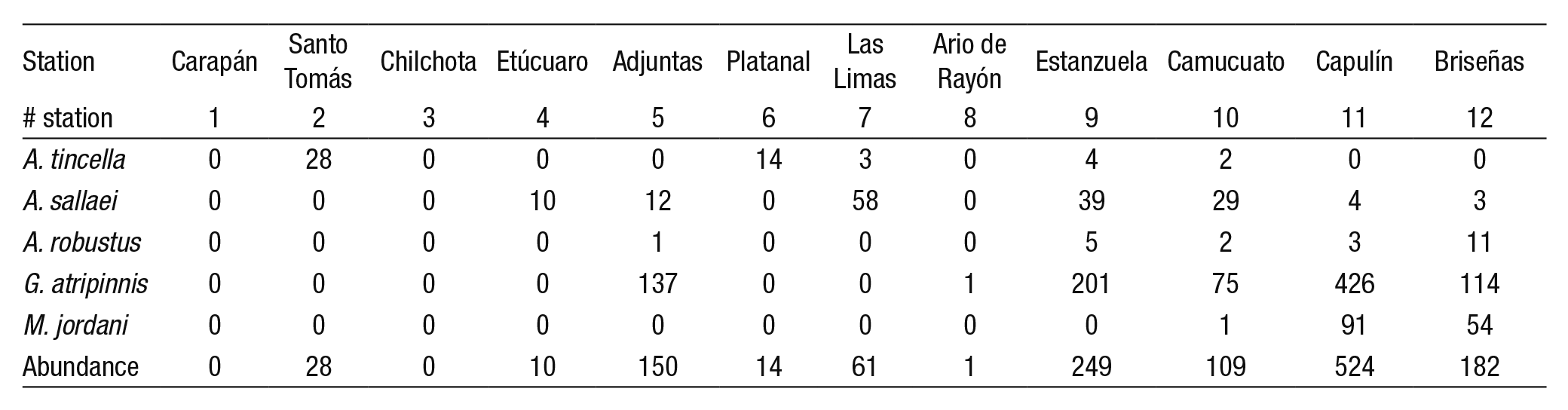
Biological sampling. As mentioned, the NMX-AA-159-SCFI-2012 (DOF, 2012) recommends using fish as target species, in order to build upon previous experience and pre-existing knowledge. For our study, we used the work of Ledesma-Ayala (1987) who had collected ichthyic species in twelve sampling sites along the whole Duero River from Ca rapan (source) to Briseñas (mouth). The structure of the fish community was analyzed by five samplings conducted from April 1985 to February 1986. More than 50% of the collected specimens (728) corresponded to the five species that we selected as indicators for the generation of suitability curves. Later, López-Eslava (1988) counted 600 specimens of the species Goodea atripinnis (also included in the suitability curves). The specimens were obtained using a seine net 20 m long by 2 m wide with a mesh size of 1/2 inch; they were immediately fixed and preserved for transportation to the laboratory (Ledesma-Ayala, 1987). Appendix 1 shows a summary of the number of species recorded by Ledesma-Ayala (1987) for each sampling site.
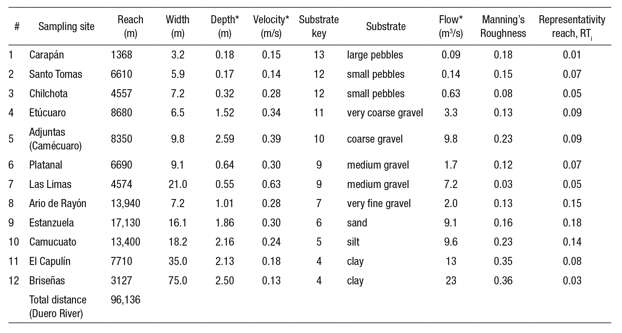
Suitability curves (Category III). These curves were generated for the following fish species: Menidia jordani, Algansea tincella, Aztecula sallaei, Goodea atripinnis and Alloophorus robustus. The procedure for genera ting suitability curves was referred to in Bovee et al. (1998) and Vargas et al. (2010). Sampling stations were characterized by relevant data (length of reach, width of river, substrate, velocity, and depth). A representation factor (RTi) was obtained from the respective distance between neighbo ring sampling sites and the total length of the river. The number of class intervals (k) was defined by Sturges’ rule, Equation (3)
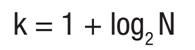 (3)
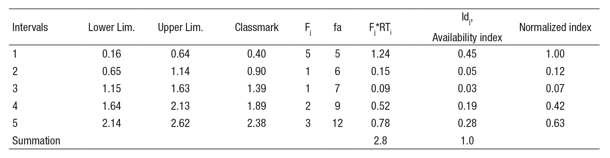
(3)Where N is the number of sampling sites (Scott, 2009). The relative frequency (Fj) was calculated for the class intervals (upper limit) for each variable: depth, velocity, and substrate. Later, Fj was multiplied by RTi. The availability index (Idj), was obtained by dividing the product (Fj)(RTi) value by the sum of total (Fj)(RTi). Additionally, each (Idj) value was divided by the maximum value of (Id). The habitat use index (Iuj) was obtained by dividing the sum of the specimens counted at each sampling site referring to each interval class; i.e., the specimens that belongs within the same class of interval are counted. Thus, stations Estanzuela (with 201) and Capulin (with 426) together sum 627 specimens of G. atripinnis, where the depth (1.86 and 2.13 m, respectively) belong to the interval # 4. Therefore, of the 627 specimens obtained it was divided by the total number of specimens (954). Then, the selection index (Cj) is calculated dividing Iuj by Idj. Finally, each value of the selection index is divided by the maximum value of Cj (see Appendix 2; example depth).
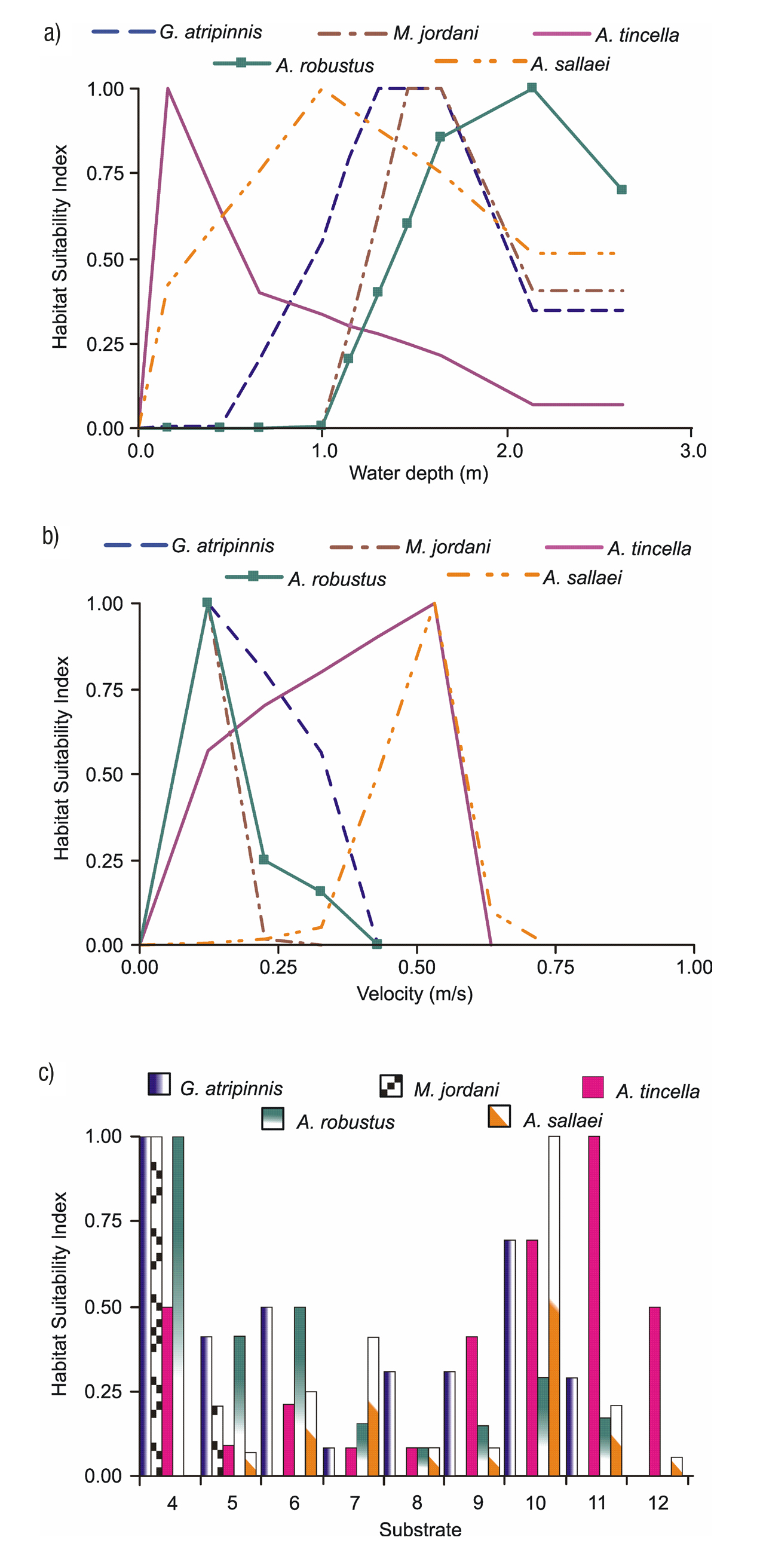
Appendices 3a-b shows the biological modeling, represented by the habitat sustainability index for the five fish species with respect to each of the habitat variables. E.g., Aztecula sallaei prefers variable depths of the water column, with depths ranging from 0.20 to 2.00 m and an optimum depth of 1.00 m. Regarding flow velocity, A. sallaei prefers ranges between 0.30 and 0.70 m/s with a suitable velocity of 0.55 m/s (but seeks higher velocities). From Appendix 3c, we observe that the same species prefers coarse substrates such as gravel, but shows a lower preference for finer gravels, sand and silt.
Model implementation. PHABSIM uses hydraulic models to calculate the water surface level (WSL) and the average velocity for each flow rate (Q) to be simulated. The WSL simulation and the hydraulic profiles were performed using the MANSQ model (Manning’s stage discharge), which uses the continuity equation (the flow volume is constant throug hout the reach) and Manning’s equation to determine the depth-flow relationship (WSL-Q) for a cross section, by assuming uniform perma nent flow conditions in each section. The velocities simulated for each section were calculated based on the velocities measured in the field by using the calibration model VELSIM (velocity simulation), which is applied when only one measured velocity profile is available (Bovee et al., 1998; Waddle, 2001).
Subsequently, calibration curves were estimated for each transect using the least squares method (regression analysis), where WSL is the dependent variable and the independent variable is Q (flow rate). The Manning’s roughness coefficient was used to calibrate these cur ves and later to calibrate the velocity distribution in PHABSIM. As only one measurement was taken, these calibration curves were used to propose other measurement points within the hydraulic section. By combining the hydraulic and biological models, the habitat availability can be quantified using the HABTAE routine of PHABSIM (Milhous et al., 1989; Moir et al., 2005; Waddle, 2001).
Appendices 4 and 5 show the calibration of the water surface level and the flow velocity (hydraulic modeling) in the “Estanz” transect (ID: 6), which is part of the upstream part of the river reach. Appendix 4a-b shows the Appendix 4 results of a minimum of three hydraulic simulations per formed with PHABSIM. The continuous line and segmented centerline represent the comparison between the observed (oWSL) and simulated (sWSL) values. The oWSL line is associated with a flow rate of 3.02 m3/s and a water-column depth of 1.30 m. The lower and upper li nes (flows of 0.5 and 11.5 m3/s), are not associated with the values measured in field, but are a function of the calibration curve of the cross section; i.e., with flow rates 0.5 and 11.5 m3/s their respective depths (0.7 and 2.6 m) and elevations (1532.7 and 1534.6 masl) were obtained. Similarly, Appendix 5a-b shows that the simulated velocity distribution sVEL is similar to the observed oVEL. For a flow of 3.02 m3/s, the average oVEL was 0.18 m/s. For flow rates of 0.5 and 11.5 m3/s average velocities of 0.08 and 0.30 m/s were obtained from the velocity distribution.
RESULTS
Alternatives to determine the optimum flow.Figure 3 shows the WUA-Q curves for the five species in the study area. Since the curve of the species Goodea atripinnis has the greatest habitat area, reaching a maximum of 4338 m2/km for a flow of 5.0 m3/s, the habitat fluctuates as a function of the flow. The Alloophorus robustus curve maintains a constant habitat of 2000 m2/km from flow of 5 to 15 m3/s. With a sma ller area, the WUA curve of Menidia jordani has a maximum habitat of 1323 m2/km for a flow of 4.5 m3/s, presenting variable behavior during flow increases.

Finally, the curves of the Algansea tincella and Aztecula sallaei species trace a smaller useful area (WUA< 500 m2/km), where the ten dency of the curves does not show increases of the area with increased flow. From these curves (WUA-Q), we derived four criteria to determine the optimum flow and thus proposed in Fig. 4 the corresponding EFR for each criterion.

1) The largest WUA curve: The curve corresponding to Goodea atri pinnis shows the greatest habitat area (4338 m2/km) with an optimum flow of 5.0 m3/s. This flow rate is representative for all five species and is set as the minimum flow during the dry season (April). According to García de Jalón & González del Tánago (1998), this situation translates into the best conditions to develop an ecological flow regime: using the natural flow curve, adjusting the optimum flow (obtained from the WUA-Q curve) by the minimum monthly value of the natural curve, and calculating the remaining months proportionally. The proposed envi ronmental flow should fluctuate similarly to the natural regime.
2) Normalizing the WUA curves: The optimum flow provides the maximum habitat percentage for all species studied herein (Leonard & Orth, 1988; Orth & Leonard, 1990). Based on the WUA-Q curves, the axis WUA was normalized by superposing the curves, generating a new habitat optimization curve, which enables the identification of an optimum flow of 5.7 m3/s corresponding to a value of 75% of the opti mum habitat. This flow, which is representative for all the species, was set as the minimum flow during April; it varied proportionally during all remaining months (similar to the previous case).
3) Maximum WUA curve: Table 3 shows the optimum flows for each species. These flows were identified from the maximum values of habitat in the WUA curves (Fig. 3). Table 4 shows the proposed monthly environmental flow regime, and the regulated flow regime to contrast monthly differences. These proposed flows represent a recovery of flows in the months of March and April for Goodea atripinnis, Menidia jordani, and Algansea tincella species, when the regulated flows are below environmental flows. Alloophorus robustus and Aztecula sallaei prefer higher flows, as in the months of April to October, while the en vironmental proposal is higher than the RFR, with the exception of July, when the regulated flow is greater than the one proposed.
Table 3 Range of optimum minimum flows for each fish species.
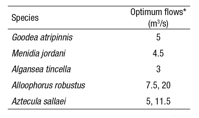
* The optimum flow was obtained from the WUA-Q curves (see Fig. 3).
4) Optimization matrix (Bovee, 1982): Table 5 shows the percen tage of the probability of exceedance of historical natural flows. With these flows (Fig. 3), the habitat (WUA) of each species is calculated. Of the five species, the minimum WUA is selected; and later, out of these values the maximum WUA is chosen (214 m2/km), which corresponds to the probability of exceedance of 50%. In other words, 7.2 m3/s is the monthly environmental flow that maximizes the habitat with the lowest contribution. This procedure was applied to the remaining months, as is shown in Figure 4. For this technique, a monthly historical series of 20 years was needed to calculate the probability of exceedance in intervals from 50 to 90%.
Table 5 Application of matrix optimization to select the average environmental flow per month (for this example, January).
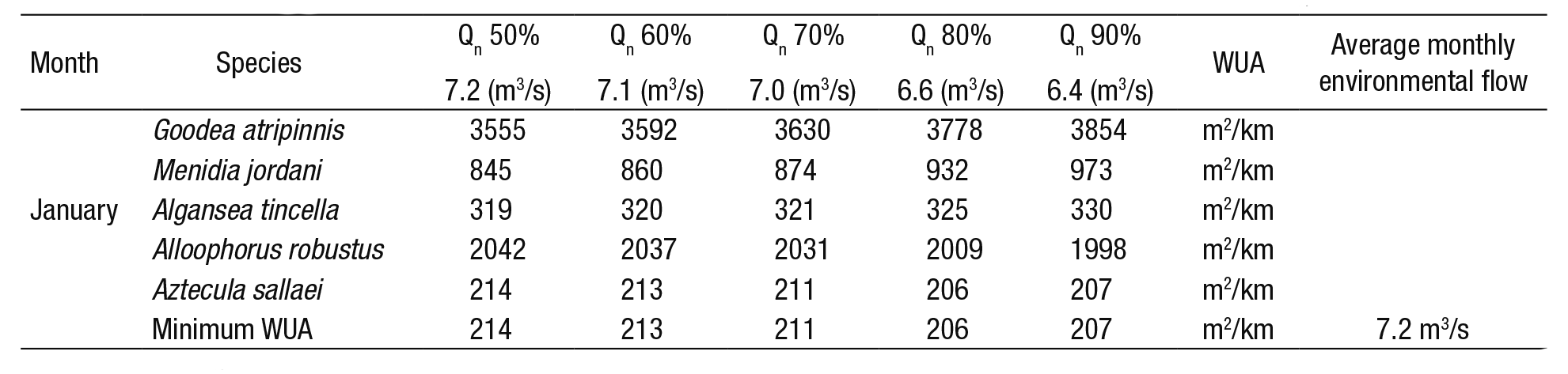
The maximum value of the minimum WUA for January is 214 m2/km and the range of natural flow (Qn) is associated with the probability of exceedance (50 to 90%).
Monthly variation of habitat.Figure 5 (left column) shows the mon thly variation of average WUA for each species: a natural WUA (flows from 1936 to 1955), a regulated WUA (1956 to 1999), and the environ mental WUA according to the optimization matrix method. The curves for Goodea atripinnis and Menidia jordani (Figs. 5a, c) show a significant difference between the regulated habitat and natural habitat in March and April. These variations of habitat oscillate between 10 and 13% for G. atripinnis and between 18 and 25% for M. jordani. The proposed environmental WUA for both species shows which of them is above the natural WUA during the dry season and which is below the natural WUA curve during the rainy season. Only Algansea tincella (Fig. 5e) displays the reverse condition where, during the dry season, the regulated WUA curve lies above the environmental and natural WUA curves (by 14%). In the rainy season, there is not much difference between the regulated and natural WUA curves. Alloophorus robustus and Aztecula sallaei experience a significant decrease of habitat in March and April with respect to the natural habitat (Figs. 5g, i). These variations range from 33 - 36% for A. robustus and 25 - 29% for A. sallaei. The environmental WUA in both species is similar to the natural WUA during the dry season. However, for A. robustus the proposed environmental WUA is 17% be low the natural habitat during the July to October rainy season.
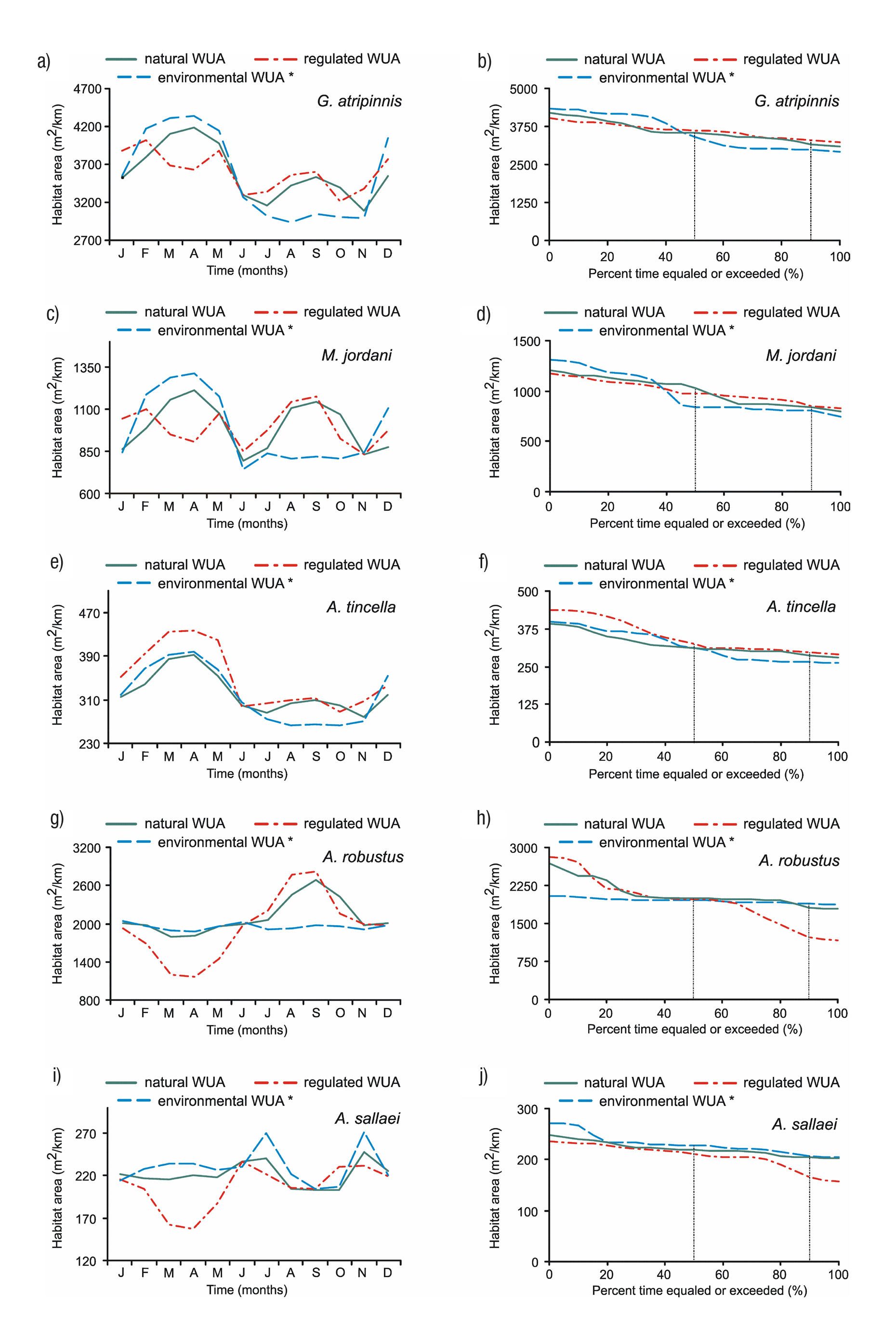
Figures 5a-j Variation in the monthly habitat (left) and habitat duration curves (right) for each fish species (* = Optimization matrix method).
Figure 5 (right column) displays the monthly behavior of the ha bitat duration curves between the natural WUA curve (reference) and the environmental and regulated WUA curves. The natural habitat for Goodea atripinnis, Menidia jordani, Algansea tincella, Alloophorus ro bustus and Aztecula sallaei more frequent or available 90% of time in an average year was 3176 m2/km, 832 m2/km, 287 m2/km, 1818 m2/km and 204 m2/km respectively (Figs. 5b, d, f, h, j). With agricultural activities in the region, the flow regime has been altered, which has had effects on the habitat of the species. Larger changes can be ob served in the habitat of A. robustus with habitat degradation of -33% and for A. sallaei with -19%.
For the other three species, minor changes in habitat duration have occurred, with +4% for G. atripinnis and A. tincella, and +2% for M. jordani.
DISCUSSION
Now that these four alternatives have been evaluated to propose EFR curves, we can confirm that all of them have acceptable behavior with respect to the NFR curve; however, only one alternative was selected for this study. By inspection, we discarded the curves obtained by the largest WUA and normalization methods, by overestimating the average natural monthly flow rates. According to Richter et al. (2003) and Thar me & King (1998), the assessment of the environmental flow of a river is to evaluate how much water of that original regime can continue to flow without compromising the integrity of ecosystems. The EFR curve (maximum WUA) has a downward behavior with respect to the natural referent curve; however, before proposing the EFR curve, not all WUA-Q curves were clear enough to identify the optimum flow for the species. According to Wilding (2007), this criterion for an inflection point is the most commonly used procedure; however, they are not always clearly present. Finally, the optimization matrix curve presented a downward behavior in the dry and rainy season, with respect to the NFR curve. According to Richter et al. (2003), it seeks a balance between the limit of the amount of water that can be withdrawn from a river and a limit on the shape to which the natural flow regime can be altered. This fourth alternative was selected to propose the environmental flow regime.
The intensive reduction of flows in the river will cause loss of habi tat for fish and other aquatic organisms (Welcomme, 1992). The flow regulation in the Duero River is mainly reflected in March and April. Con trasting the habitat variation curves, Figure 5 (left column) shows that the flow regulation has affected four of the five fish species. We should note that Goodea atripinnis and Menidia jordani have decreased habitat from March to April, partially affecting the reproductive period of both; however, the reproduction period of G. atripinnis has been extended from April to September (Barragán & Magallón, 1994) and from February to August for M. jordani (Miller et al., 2009). Despite this partial affecta tion of habitat, Lyons et al. (1995, 2000), Mercado-Silva et al. (2006) and Ramírez-Herrejón et al. (2012) depict both species as tolerant of environ mental degradation, being prolific species with an annual presence. The preferred habitat of both species occurs in the dry season, with optimum minimum flow of 4 to 5.5 m3/s; however, they also adapt well to flow rates in the rainy season (between 18 to 20 m3/s). The proposed environ mental WUA curve (optimization matrix method) shows a slight increase in habitat during the dry season and decreased habitat during the rainy season, indicating a probable natural limit.
River regulation resulted in more habitat decline from January to May for Alloophorus robustus and Aztecula sallaei, affecting various stages of life. E.g., the juvenile stage of A. robustus is from February to March. The spawning period of A. sallaei is from February to April, and maybe until May (Miller et al., 2009), and the reproduction period lasts from April to August for A. robustus (Mendoza, 1962; Soto-Galera et al., 1990) and from March to September for A. sallaei (Sánchez & Navarrete, 1987). Considering the habitat duration curves, the contrast between NFR and RFR was evident for 50% of the time. The useful habitat of both species is mostly in the rainy season; though with a different range of the optimum minimum: 7.5 to 20 m3/s for Alloophorus robustus and 5 to 11.5 m3/s for Aztecula sallaei. However, both species also find favorable habitat in the dry season, while Alloophorus robustus is normally found in lentic water and Aztecula sallaei prefers moderate to strong currents (Miller et al., 2009). According to Lyons et al. (1995, 2000), Mercado-Silva et al. (2006), and Ramírez-Herrejón et al. (2012), both species are sensitive or intolerant towards habitat deterioration.
Finally, regarding Algansea tincella, with medium tolerance status (Lyons et al., 1995, 2000; Mercado-Silva et al., 2006; Ramírez-Herrejón et al., 2012), the available habitat area has increased with flow regulation and life stages (spawning and reproduction) do not seem to be com promised, but the reproduction season in April benefits from regulation. According to Welcomme (1992) the aquatic organisms in rivers usually adapt to the regimes of the flow. The preferred habitat of Algansea tin cella is at the flow rates that corresponding to the dry season, with an optimum flow of 3 to 4 m3/s; however, it also prefers 8 m3/s in the rainy season (November). As for the proposed EFR, the habitat in the rainy season decreases below the natural reference, which can be considered a new limit capable of maintain the integrity of the ecosystem.
EFR proposal. Figure 6 shows the proposed environmental flow requi rement, the regulated flow regime (RFR) and the minimum regulated flow regime (mRFR) in order to compare the monthly flow variation. In the dry season, environmental flows from January to May are greater than the regulated flow (RFR curve), being March and April the most critical with RFR at 30% below the environmental proposal. According to García de Jalón & González del Tánago (1998), the environmental flows must be greater in periods of low flow. In the rainy season, the EFR curve shows an increasing trend from June to August, reaching a maximum in September and decreasing from October to November. According to Richter et al. (2003), there are limits to the amount of water that can be withdrawn from rivers before severely degrading their natural functions and the services they provide.
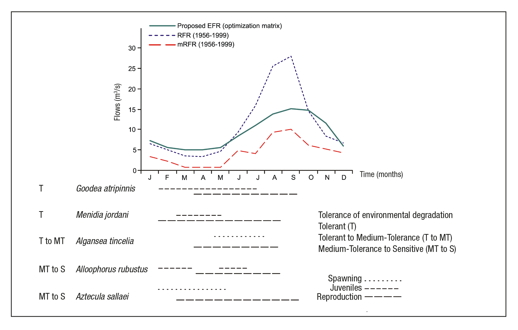
Figure 6 Proposal environmental flow requirement (EFR) in the study area, contrasting with flows regulated and life stages. Note: The life stages with information: Barbour & Miller (1978), Barragán & Magallón (1994), Ledesma-Ayala (1987), López-Eslava (1988), Mendoza (1962), Miller et al. (2009), Navarrete & Sánchez (1987) and Soto-Galera et al. (1990). Tolerance of environmental degradation with information from Lyons et al. (1995, 2000), Mercado-Silva et al. (2006) and Ramírez-Herrejón et al. (2012).
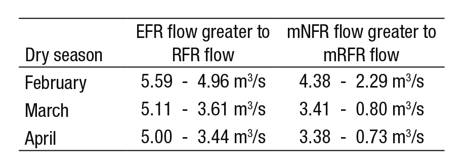
The average annual flow rate under the NFR is 11.36 m3/s, for re gulated flow it is 10.98 m3/s and for the proposed EFR it is 9.09 m3/s. From this we can assume that annual regulation has not significantly affected the flow behavior of the river, reported at only 5% below natural conditions (NFR curve). However, with monthly regulation (during the dry season), the data shows a different perspective. Figure 6 now shows that the proposed EFR lies above the RFR curve from January to May (e.g., see Table 6). During the dry season, the current average flow rates (RFR cur ve) resemble the conditions of the mNFR curve; i.e., the minimum flows during the natural regime. Consequently, the minimum regulated flows (mRFR) have reached levels not yet registered in the 1936-1955 period. For example, Table 6 shows the variation of February, March, and April.
Table 6 Comparison between flows: environmental vs regulated, and natural minimums vs regulated minimums.
García de Jalón & González del Tánago (1998) point out that the flow and habitat requirements of different fish species can vary widely throughout the year. In case of the Duero River, Alloophorus robustus and Aztecula sallaei require greater flow rates during the dry season, implying loss of habitat and stress to their life stages (spawning and reproduction, Fig. 6). The proposed environmental flow regime can be nefit their life cycle, due to the natural tendency of the proposed curve. In other words, if the habitat is unfavorable to these species, Algansea tincella finds it favorable. Similarly, Goodea atripinnis and Menidia jor dani found favorable habitat and flows throughout the year.
Regulation on the Duero River resulted in an average annual varia tion of less than 10% between the natural (NFR, 1936-1955) and the regulated flow regime (RFR, 1956-1999); for the annual average mini mum flow (mNFR and mRFR curves) this difference was 40%. Howe ver, looking at monthly data, during the dry season from January to May the difference between the minimum flows (regulated vs natural) was a 66% decrease; showing that the effect of the regulation is most noticeable in the dry season. The difference between the annual ave rage NFR curve and the EFR curve is 20%; i.e., the environmental flow preserves up to 80% of the natural flow regime. This EFR proposed for the lower reach of the Duero River during the dry season generates a favorable effect on the available habitat areas of the five target fish species, with a 11% increase of WUA for A. tincella, and a recovery of degraded habitat area for G. atripinnis (with 10%), M. jordani (18%), A. robustus (24%) and for A. sallaei (23%).
The management of environmental flows should be a fundamental part of the integrated water resources management approach in the Duero River, due to its beneficial mitigation impacts on the constant pressure of regulatory activity. It would be convenient to discontinue decreasing this activity from March and April (3.61 to 3.44 m3/s), thus avoiding the occurrence of minimum regulated flows; we also recom mend establishing the proposed average environmental flows from 5.11 to 5.00 m3/s (for March and April, respectively).
The regulation of the river has direct implications on the available habitat of the target species, mainly in March and April; Alloophorus robustus and Aztecula sallaei are the most affected, while Algansea tincella benefits with an increase in habitat. However, in the rainy sea son regulation has not affected the habitat of the species. We should mention that this analysis of the habitat variation curves was done with monthly average information. Thus, it is necessary now to analyze habitat variation with minimum flows. Flow rates lower than 1 m3/s during March, April, and May increase habitat degradation in the river and diminish ecosystem resilience. With an environmental proposal of 80% conservation of the NFR, we recommend identifying other lower thresholds to observe the variation in the fluvial habitat.
We believe that this research will be relevant at the national level, since it is one of the first studies to apply this methodology to a Mexican river. The study focuses on only one reach of the river, on the lower basin where the instream water demand competes with irrigation in frastructure. Therefore, water management plays an important role in the allocation and/or implementation of environmental flows, for care and conservation of the aquatic ecosystems in the DRB.