


Servicios Personalizados
Revista

Articulo
 Inglés (pdf)
 Artículo en XML
 Referencias del artículo
 Enviar artículo por email
Indicadores
 Citado por SciELO
 Links relacionados
-
 Similares en
SciELO
Similares en
SciELO
Compartir

 Permalink
Hidrobiológica
versión impresa ISSN 0188-8897
Hidrobiológica vol.21 no.3 Ciudad de México sep./dic. 2011
Elements of support to estimate total and new primary production in the Gulf of California based on satellite data
Elementos de apoyo para estimar la producción primaria total y nueva del Golfo de California basada en datos de satélite
Saúl Álvarez-Borrego
Department of Marine Ecology, Division of Oceanology, CICESE, Carretera Ensenada-Tijuana No. 3918, Zona Playitas, Ensenada, Baja California, 22860. México. e-mail: alvarezb@cicese.mx
Recibido: 20 de junio de 2011.
Aceptado: 7 de octubre de 2011.
ABSTRACT
High rates of primary production support the great animal biodiversity of the Gulf of California. One of the main limitations to estimate total (PT) and new (PNEW) primary production by 14C and 15N bottle incubations, respectively, is the small number of point samples generated for a particular area, and with very poor time coverage. Satellite ocean color sensors offer an alternative to estimate phytoplankton production rates in the oceans with an ample spatial-temporal variability that is not possible to cover with research vessels. With ocean color sensors in orbit, scientific expectations remain to improve ocean primary production models. Parameters used by these algorithms fall into three categories: environmental, ecological, and physiological. A review is given on studies that have generated information on these parameters for Gulf of California waters, and opportunities for new research are highlighted. Satellite surface pigment (Chls) and irradiance data (PARsat) need to be associated to vertical profiles (Chlz and PARz) generated with a Gaussian distribution function and Lambert-Beer's law, respectively. A detailed description is given of the parameters that characterize this Gaussian function and a vertical attenuation coefficient of PAR variable with z, for different seasons and regions within the Gulf of California. The weakest part of modeling primary production are the photosynthesis-ir-radiance (P-E) curve parameters: the initial slope, assimilation number, and quantum efficiency, and these give us an opportunity for new research. Summer data to characterize all the set of parameters needed for modeling primary production based on satellite data are the scarcest.
Key words: Gulf of California, satellite ocean color sensors, modeled primary production, pigment and irradiance profiles parameters, photosynthesis-irradiance parameters.
RESUMEN
La gran biodiversidad animal del Golfo de California es producto de su elevada producción primaria. Una de las principales limitaciones para estimar la producción primaria total (PT) y nueva (PNUEVA) mediante incubaciones con 14C y 15N, respectivamente, es el pequeño número de muestras puntuales generadas para un área en particular, y con cobertura temporal muy pobre. Los datos de satélite ofrecen una alternativa para estimar la producción fitoplanctónica del océano con una variabilidad espacio-temporal grande que no es posible cubrir con barcos oceanográficos. Con sensores de color del océano en órbita, se tienen altas expectativas científicas de mejorar los modelos de producción primaria oceánica. Los parámetros usados por estos algoritmos son de tres tipos: ambientales, ecológicos y fisiológicos. Se hizo una revisión de los estudios que han generado información sobre estos parámetros para las aguas del Golfo de California, y se indican las oportunidades de nuevos proyectos de investigación. Se requiere asociar los datos superficiales de satélite de pigmentos (Chls) e irradiación (PARsat) con los perfiles verticales (Chlz y PARz) generados con una distribución Gausiana y la ley de Lambert-Beer, respectivamente. Se da una descripción detallada de los parámetros que caracterizan esta función Gausiana y de un coeficiente de atenuación vertical de PAR variable con z, para diferentes estaciones y regiones del Golfo de California. La parte más débil del modelado de la producción primaria son los parámetros de la curva fotosíntesis-irradiancia (P-E): la pendiente inicial, el número de asimilación y la eficiencia cuántica, lo cual representa una oportunidad para nuevos proyectos de investigación. Los datos más escasos son los que caracterizan todo el conjunto de parámetros para modelar la producción primaria basada en las imágenes de satélite de verano.
Palabras clave: Golfo de California, imágenes satelitales de color, producción primaria modelada, parámetros de los perfiles de pigmentos e irradiancia, parámetros de la curva fotosíntesis-irradiancia.
INTRODUCTION
Few places in the world can claim such a diversity of species as the Gulf of California, with its 6,000 recorded animal species estimated to be half the number actually living in its waters. Over half-million tons of seafood is taken from it annually. The accumulation of species diversity, since the Gulf's opening ~5.6 million years ago, has produced one of the biologically richest marine regions on earth (Brusca, 2010). This great biodiversity is supported by high rates of primary production. The Gulf of California has three main natural fertilization mechanisms: net water exchange with the Pacific, upwelling, and mixing by winds and by phenomena associated with tides (Álvarez-Borrego, 2010). Upwelling occurs off the eastern coast with northwesterly winds ("winter" conditions from December through May), and off the Baja California coast with southeasterly winds ("summer" conditions from July through October), with June and November as transition periods (Álvarez-Borrego & Lara-Lara, 1991). With northwesterly winds upwelling is strong, it has a marked effect on phytoplankton communities (surface chlorophyll a concentration, Chls, values up to >10 mg m-3), and due to eddy circulation it increases the phytoplankton biomass across the Gulf (Santamaría-Del-Angel et al., 1994). However, because of strong stratification during summer, upwelling with southeasterly winds has a very weak effect on phytoplankton biomass (Santamaría-Del-Angel et al., 1999).
New primary production (PNEW) is the fraction of primary production (PT) supported by the input of nitrate from outside the euphotic zone (Dugdale & Goering, 1967), mainly from below the thermocline by vertical eddy diffusion (Eppley, 1992). It is an estimate of oceanic particle flux in the global carbon cycle (Eppley & Peterson, 1979). Phytoplankton cells use nutrients recycled within the euphotic zone for regenerated production (Pr). Total production is equal to the sum of both new and regenerated production (PT = PNEW + Pr). Eppley & Peterson (1979) defined the ratio of PNEW to PT as the f-ratio (f= PNEW/PT) and showed that f is an asymptotic function of the magnitude of PT. The description of the temporal and spatial variability of PNEW may give us an idea of the variability of the flux of organic matter out of the surface layer. However, one of the main limitations to estimate PT and PNEW by 14C and 15N bottle incubations, respectively, is the small number of point samples generated for a particular area, and with very poor time coverage. Thus, satellite ocean color sensors offer an alternative to estimate the phytoplankton primary production rates in the oceans with an ample spatial-temporal variability that is not possible to cover with research vessels.
The processesoffixation of inorganic carboninorganic matter during photosynthesis, its trophodynamic transformation, physical mixing, transport and gravitational settling are referred to collectively as the ''biological pump'' (Ducklow et al., 2001). The ratio of sinking flux to primary production (e-ratio) and the f-ratio depend on the pathways by which nitrogen flows among different organisms (phytoplankton, large and small grazers and bacteria), but the only way to change the absolute amount of export is to change PNEW, which is usually controlled by physical factors (Frost, 1984).
Satellite-derived estimates of basin-scale and global-scale primary production have been performed (i.e., Sathyendranath et al., 1991; Longhurst et al., 1995). The approach used is based on partition of the ocean into a suite of domains and provinces within which physical forcing, and the algal response to it, are distinct (Platt et al., 1991). Empirical and semianalytical algorithms to estimate primary production from photosynthetic pigment concentration have been developed (i.e., Behrenfeld & Falkowski, 1997). Usually the objective is not to obtain instantaneous local rates of production, but rather to calculate primary production for relatively large geographic areas and for periods of months. With ocean color sensors in orbit, high expectations remain to improve ocean primary production models (Behrenfeld et al., 1998; Hidalgo-Gonzalez & Álvarez-Borrego, 2004). Parameters used by these algorithms fall into three categories: environmental (e.g., location, atmospheric conditions, the irradiance vertical profile); ecological (e.g., the chlorophyll a concentration (Chlz) vertical profile); and physiological (e.g., the photosynthesis-irradiance (P-E) curve parameters, the chlorophyll-specific absorption coefficient of phytoplankton (a*ph(λ)), photosynthetic quantum yields (ϕz) (Morel, 1991).
A primary goal of a production algorithm is to observe variability in oceanic values occurring on time scales up to interannual-to-decadal and regional-to-global space scales. It is impossible to observe variability at these scales by any means other than by satellite (Behrenfeld et al., 1998). We are interested in improving the precision of primary production estimates at the global scale, and also in generating primary production time series for particular regions of the ocean that could be applied to, for example, oceanographic fisheries studies. Studies to generate information on the parameters involved in the calculations of primary production in Gulf of California waters have been performed (Álvarez-Borrego & Gaxiola-Castro, 1988; Valdez-Holgufn et al., 1999; Gaxiola-Castro et al., 1999; Giles-Guzmán & Álvarez-Borrego, 2000; Cervantes-Duarte et al., 2000; Hidalgo-Gonzalez & Álvarez-Borrego, 2001), but more data are needed to improve the characterization of parameters involved in estimating primary production for the Gulf based on ocean color. Opportunities for new research will be highlighted.
GENERAL CONSIDERATIONS
Early models to estimate primary production in the ocean were based on laboratory experiments to characterize the photosynthesis-light relationship (Ryther, 1956; Ryther & Yentsch, 1957). They offered the basis for models that make use of variables measured from remote sensors (e.g., pigments, irradiance, etc.) (Platt & Sathyendranath,1988; Longhurst et al., 1995; Behrenfeld & Falkowski, 1997; Hidalgo-Gonzalez et al., 2005). PT is given pixel-by-pixel as a standard product in the NASA web page (http://oceancolor.gsfc.nasa.gov/) calculated from satellite chlorophyll a concentration (Chlsat), sea surface temperature (SST), and scalar photosynthetically active radiation, 400-700 nm, (PARo(sat)) using Behrenfeld and Falkowsky's (1997) vertically generalized production model (VGPM) (Behrenfeld et al., 1998). The VGPM is a non-spectral, homogeneous-biomass vertical distribution, vertically integrated, production model. This means that chlorophyll and the quality of light are not allowed to change with depth, and this causes inaccuracy. Furthermore, there are no data for the Gulf of California on the parameters used by this model: Pbopt (the photosynthetic ratio or photosynthesis per unit Chl at the optimum light level in the water column) (mgC mgChl-1 h-1), and f(PARo) (a function that represents the effect of light in the whole euphotic zone and throughout the whole day). As a first approximation, representative values for these parameters are used for large oceanic provinces and for the whole year. A better approximation to reality is to generate the PTz (mg C m-3 h-1) vertical profile (with a PTz value for each meter) with the model proposed by Platt et al. (1991), or its modification proposed by Hidalgo-Gonzalez & Álvarez-Borrego (2004). Platt et al.'s (1991) model is a non-homogenous, non-spectral model, and this means that Chl is allowed to change with depth (Chlz) by means of a Gaussian curve that reproduces the deep chlorophyll maximum, but the change of the spectral distribution of PARz with depth is not taken into consideration. Hidalgo-Gonzalez & Álvarez-Borrego's (2004) modification is a non-homogeneous, spectral model that allows for the change of the spectral distribution of irradiance with depth, based on the method proposed by Giles-Guzmán & Álvarez-Borrego (2000).
In the context of remote sensing, a classification which has been found useful divides oceanic waters into "Case I" and "Case II" waters (Morel & Prieur, 1977; Gordon & Morel, 1983). Case I waters are those for which phytoplankton and their derivative products (organic detritus and colored dissolved organic matter (CDOM), arising by zooplankton grazing, or natural decay of algal cells) co-vary and play a dominant role in determining the optical properties of seawater. Case I waters have Chlz <1.5 mg m-3. Case II waters are those for which the above mentioned optical components of seawater do not co-vary, and also an important or dominant contribution to the optical properties of seawater may come from inorganic suspended matter or material carried by river runoff. Case II waters have Chlz >1.5 mg m-3.
Platt et al.'s (1991) model has been used for Gulf of California case II waters:
where: the asterisk means that the value is normalized per unit of chlorophyll a concentration; P*m (mg C (mg Chl)-1 h-1) is the photosynthetic rate at saturating irradiance or assimilation number; Chlsat(z) is the average Chl for depth z for a whole season and region within the Gulf, derived from the satellite data (Chlsat) and a model for the Chl vertical distribution; α*PAR (mg C (mg Chl)-1 h-1 (μmol quanta m-2 s-1)-1) is the initial slope of the photosynthesis-irradiance (P-E) curve; and PARz (umol quanta m-2 s-1) is PAR for depth z, derived from the satellite data (PARo(sat)) and Lambert-Beer's law with a constant vertical attenuation coefficient of diffuse light (KPAR).
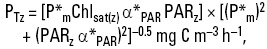
Hidalgo-Gonzalez & Álvarez-Borrego (2004) used a modification of Platt et al.'s (1991) model for Gulf of California case I waters:

In this equation Φmax is the maximum quantum yield (mol C (mol quanta)-1), and a*ph(Z,ch) (m2 (mg Chl)-1) is the phytoplankton specific absorption coefficient of light averaged for the spectral distribution of PAR at depth z. This corrects the initial slope α*PAR for the spectral distribution of the in situ scalar PAR. In place of α*PAR the product 43.2Φmax a*ph(Z,chl) was used (Giles-Guzmán & Álvarez-Borrego, 2000). The factor 43.2 converts mol C to mg C, seconds to hours, and mol quanta to umol quanta. These expressions show that to estimate PTz, not only the surface Chl value is needed, but also the vertical profiles of Chl and PAR. In this case PARz is derived from the satellite data (PARo(sat)) and Lambert-Beer's law with a variable vertical attenuation coefficient of diffuse light (KPAR(chl,z)) as a function of Chlz and depth.
Algorithms to transform the optical satellite data into products like Chlsat need "ground truth" data from oceanographic cruises. There is the perception that instantaneous point PT estimates based on satellite data are very imprecise and inaccurate because the development of satellite algorithms are based on calibration cruises that cover limited portions of the ocean. But when the average of satellite data are used for whole oceanic regions, and for relatively large time scales, such as months or seasons, the estimated PT values can very well represent the biological dynamics of those regions (Hidalgo-Gonzalez & Álvarez-Borrego, 2004). The large number (n) of pixels within our region of interest, and for whole months, allows for very precise pigment (Chlsat) and PARsat averages with relatively small standard errors (s/n0.5) (Hidalgo-Gonzalez & Álvarez-Borrego, 2004). Morel & Berthon (1989) indicated that it is unreasonable and probably superfluous to envisage the use of a light-production model on a pixel-by-pixel basis when interpreting satellite imagery. Furthermore, some of the satellite calibration cruises have been carried out in the Gulf of California where personnel from CICESE and the Autonomous University of Baja California have participated on board UNAM's R/V El Puma (1993) and SIO-UC's R/V Melville (1999). The Gulf of California provides with cloudless skies needed for calibration cruises, and this results in relatively accurate satellite products for the gulf.
The vertical distribution of chlorophyll. Satellite data collection is limited to electromagnetic radiation. Thus the oceanographic information is restricted to the immediate surface layer of the ocean. Remotely sensed ocean color is limited to a depth at which 90% of the backscattered solar irradiance from the water column originates. Remote sensors provide information on the sui generis average photosynthetic pigment concentration for the upper 22% of the euphotic zone (Kirk, 1993). Primary production models apply to the entire euphotic zone, and ideally, they should use the vertical profile of pigment biomass as input. Therefore a gap exists between the limited satellite information and what is needed when modeling.
The assumption of a mixed layer with a homogeneous pigment distribution could lead to inaccurate estimates of integrated primary production (Platt et al., 1991). The deep chlorophyll maximum (DCM) is a consistent feature in the ocean. Generally, accounting for its presence increases estimates of integrated primary production, and since the DCM often appears below the mixed layer it would be likely that most of its primary production is new production (Sathyendranath et al., 1995). In the Gulf of California the DCM coincides with the upper part of the nitracline, where nitrate concentration is >1.0 (Cortes-Lara et al., 1999). Lewis et al. (1983) proposed a Gaussian distribution function to represent the vertical profile of chlorophyll concentration (Chlz) (Fig. 1). A difficulty in estimating oceanic primary production from surface measurements arises from the regional differences in the vertical distribution of Chlz. Therefore it is necessary to use Chlz historical data to characterize the parameters of this Gaussian function for each oceanic province or region.
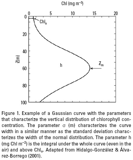
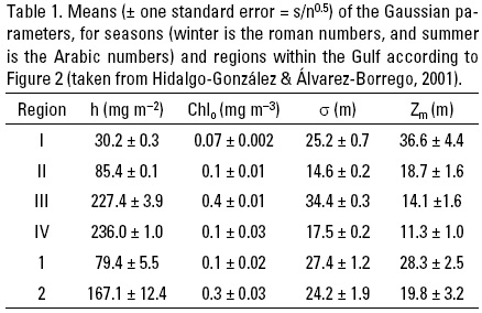
Following Lewis et al. (1983), Hidalgo-Gonzalez & Álvarez-Borrego (2001) used chlorophyll concentration (Chlz) historical data to fit a Gaussian distribution function to represent the pigment vertical profile for different seasons and regions within the Gulf of California. As a first approximation, we can represent Chlsat by the Chlz average for the first optical depth, weighted by the irradiance attenuated twice (when the light is going down and when it is backscattered up) (Kirk, 1993). For the available Gulf of California in situ Chlz data, the Chlz weighted average for the first optical depth is about 10% higher than the surface Chl (Chls), thus Chls = 0.9Chlsat (Hidalgo-Gonzalez & Álvarez-Borrego, 2001). Gulf of California Chlz profiles were fitted to Lewis et al. (1983) equation: Chlz = Chlo + [h/(α(2π)0.5)]exp[-1/2(Z - Zm)2/α2], where Chlo is the background chlorophyll concentration (mg m-3), h is the total chlorophyll (mg m-2) above the baseline Chlo, α controls the thickness of the DCM layer (m), and Zm is the depth of the maximum (Fig. 1). Hidalgo-Gonzalez & Álvarez-Borrego (2001) used 268 chlorophyll concentration profiles to estimate these parameters. These latter authors used cluster analysis of surface temperature to define the cool season for the Gulf of California as the period between end of November-end of June, and the rest of the year is considered the warm season. However, to be consistent with the previously defined "winter" and "summer" conditions, with November and June as transition periods, and recognizing interannual variability, Hidalgo-Gonzalez & Álvarez-Borrego (2001) followed Valdez-Holgufn et al.'s (1999) criteria and considered mean surface temperatures of <24 ºC as indicative of cool season. Surface temperatures <24 ºC indicate either strong mixing or the start of upwelling events off the east coast. Cluster analysis of surface temperature and chlorophyll data grouped the stations into four regions for the cool season and into two regions for the warm season (Fig. 2). The warm season data are less abundant (only 48 profiles) and show less horizontal structure in the Gulf. The four regions for the cool season coincide very closely with those proposed by Gilbert & Allen (1943) based on the abundance of phytoplankton during winter-spring.
During both seasons, h significantly increased from south to north (Table 1). Lowest h mean value was 30 mg m-2, for region I, and highest value was 236 mg m-2, for region IV (Table 1). Values for the parameter h are higher than integrated chlorophyll for the euphotic zone because h values include the whole area under the Gaussian curve. Regions II and IV had very different h values with very similar a and Chlo values because of different average Chl values at the DCM (Chlm). In the cool season, Chlo increased slightly from region I to region II (0.07 to 0.11 mg m-3), then it had a relatively high value in region III (0.39 mg m-3) and decreased in region IV to a value similar to that of region II (0.14 mg m-3). In the warm season, Chlo increased northward (Table 1). The mean of a did not have a monotonic pattern of geographic change in the cool season. Its range was 14.6-34.4 m. During the warm season, a had values similar to the one for region I, with no significant difference between regions 1 and 2 (Table 1). Relatively few of the profiles (~15%) had surface maxima (Zm = 0 m), and none of these were in regions I and 1. The mean depth of the DCM, Zm, showed a clear tendency to decrease from south to north in the cool season (from 36.6 to 11.3 m), but this tendency was not as strong in the warm season (28.3 to 19.8 m) (Table 1). Due to the scarcity of data from the Gulf of California, Hidalgo-Gonzalez & Álvarez-Borrego (2001) were not able to build regression models to predict the parameters h, Chlo, α, and Zm as functions of remotely sensed variables such as Chlsat and SST. Thus, they proposed to use means of Chlo, h, and a, for each region and season (Table 1), to calculate the representative Chlz profile. There are two alternatives to estimate Zm. One is to use the mean of Zm for each region and season, but this leaves no degrees of freedom for the use of satellite imagery. Thus, a better alternative to estimate Zm is to use the Gaussian equation and the mean value of Chlsat for the chosen region and season of the particular year. Thus:

The Zm values derived from this latter equation are practically the same as those derived directly from the chlorophyll profiles (Hidalgo-Gonzalez & Álvarez-Borrego, 2001). It is important to notice that a single Chls value produces different Chlz profiles for the different regions and seasons. However, there is an opportunity for new research because more Chlz profiles are needed to better characterize the Gaussian parameters for the "summer" season. With only 48 "summer" profiles the spatial coverage is very poor.
The vertical attenuation coefficient of PAR (KPAR). Bio-optical models to estimate primary production in the ocean, based on analysis of P-E curves, are mathematically tedious but give predictive capability by permitting continuous calculation of primary production based on the rate of light absorbed (Falkowski & Raven, 1997). Part of the tediousness arises from the decomposition of parameters and variables into spectral components, and from their variation with the composition of seawater (e.g., PAR (λ, z), aph(λ, z), KPAR(λ, z)). It would be much better if biological oceanographers could do the computations using single values for in situ scalar PAR (PARz), and for an average of aph(λ, Z) (aph(PAR, z)). This average should be weighted by the shape of the in situ spectrum of PAR.
The universal bio-optical algorithm of the Coastal Zone Color Scanner (CZCS) for case I waters (Gordon et al., 1983) implicitly contains an average covariance of the absorption by phyto-plankton and CDOM and detritus in surface and near surface waters. That covariance was made explicit by combining the CZCS algorithm with an expression for reflectance. Case I waters are more than 95% of the ocean. The spectral variation of absorption by CDOM plus detritus for case I waters may be estimated by the expression: agd = 2a*ph(440)Chl{exp[-0.013(λ-440)]} (Giles-Guzmán & Álvarez-Borrego, 1996). Based on this expression, and data and empirical models found in the literature for the absorption of phytoplankton and pure seawater (Cleveland, 1995; Pope, 1993), Giles-Guzmán & Álvarez-Borrego (2000) deduced an expression to estimate the average coefficient of total absorption for case I waters, for the whole visible range, weighted by the spectral distribution of PAR at depth, as a function of Chl and L (length of the mean trajectory of light):
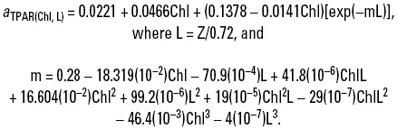
Giles-Guzmán & Álvarez-Borrego (2000) also used an empirical expression for the scattering coefficient (Gordon & Morel, 1983) and data on the volume scattering function (Petzold, 1972) to deduce an expression for the average backscattering coefficient and for the visible range, weighted by the in situ spectral distribution of PAR, as a function of Chl: bbPAR(Chl) = 0.019[0.0015 + 0.3(Chl)0.62]. Preisendorfer's (1961) expression can be used with aTPAR(Chl, L) and bbPAR(Chl) to estimate KPAR(chl, L), the vertical attenuation coefficient of PAR for case I waters (KPAR(Chl, L) = (aTPAR(Chl, L) + bbPAR(Chl))/μd). Giles-Guzmán (1998) showed that a satisfactory choice for μd, the average cosine for downwelling light, is to follow Zaneveld et al.'s (1997) suggestion and set μd invariable with depth and equal to the value for the asymptotic region, μd(α) = 0.72. If we know the Chl vertical profile and the irradiance incident at the surface (PARsat), the vertical profile of scalar irradiance (PARz) may be calculated. Following Morel & Maritorena (2001), PARsat is multiplied by 0.965 to estimate PAR immediately under the sea surface (PARz = 0-), and then Lambert-Beer's law is applied with a variable KPAR(Chl,L) to generate the PARz profile.
Average surface chlorophyll (Chls) for whole seasons and regions within the Gulf is usually <1.5 mg m-3, but due to the DCM in some cases Chlz is >1.5 mg m-3. In those cases, the PARz profile for the near surface waters (with Chlz <1.5 mg m-3) is calculated following Giles-Guzmán & Álvarez-Borrego (2000), and the PARz profile for deeper waters (with Chl >1.5 mg m-3) is calculated with Lambert-Beer's law and an average vertical attenuation coefficient, KPAR, deduced from the satellite K490 average value (K490 is another product deduced from the satellite sensor's data and provided by NASA). The regression models proposed by Cervantes-Duarte et al. (2000) (ZPAR1% = A + B/K490) are used to estimate the euphotic zone depth (Zeu) as a function of K490 in each case, and KPAR is estimated (KPAR = 4.6/ZPAR1%). The regression parameters A and B have different values for different regions within the Gulf (A = -5.12, B = 5.31 for the northern basin; A = 5.6, B = 4.24 for the midriff islands region; and A = 16.21, B = 3.13 for the southern basins). Data used by Cervantes-Duarte et al. (2000) were collected during cruises carried on during autumn and winter only, and hydrostations were occupied mostly at and near the Guaymas basin, with few locations in the northern and southernmost basins, and this gives an opportunity for future research to better characterize this kind of regression parameters (A and B) for all seasons and regions of the Gulf.
THE PHYTOPLANKTON PHYSIOLOGICAL PARAMETERS
At least one liter of water sample is filtered through GF/F glass-fiber filters for ap (λ) measurements. Particle absorption is measured with a spectrophotometer equipped with an integrating sphere to include all scattered light. A second reading is obtained after extraction of pigments with hot methanol following Kishino et al. (1985), to determine detrital absorption (ad(λ) and the difference is phytoplankton pigment absorption: aph(λ) = ap(λ) - ad(λ)*. Raw absorbances (optical densities, OD) are corrected for the path-length amplification effect (β factor, due to light scattered inside the filter) by using algorithms empirically derived from laboratory cultures (Valdez-Holgufn et al. 1999).
A photosynthesis-irradiance (P-E) curve is constructed by plotting PT normalized per unit Chl (P* mg C mg Chl-1 h-1) versus PAR (Fig. 3). To generate the P-E curves phytoplankton samples are taken from a number of predetermined depths, each water sample is passed through a 333-μm mesh to remove large herbivores, and then incubation experiments are run with n aliquots from each sample. Before incubating, 14C is added to each aliquot to a final concentration (usually 0.5 μCi mL-1, but it depends on Chl), and then incubated for one or two hours under a light gradient. The latter has been done either with the natural sun light (using neutral screens to simulate the in situ light levels) or in incubators with lamps. Generally, temperature is maintained within 3 °C of in situ temperature. Additional aliquots are used for dark incubation and for a time-zero control; the latter are immediately acidified after filtration. After incubation, the samples are acidified and then filtered. Radioactivity is determined with a scintillation counter and carbon assimilation estimated usually following Strickland & Parsons (1972). Productivities per unit Chl are calculated (P*) and plotted versus the incubator's irradiances. The initial slope of the P-E curve, α*, is determined with a linear regression of the low irradiance points (this is α* for the incubator's light, α*inc). To estimate the maximum P* or assimilation number, P*m, the data are fitted to Smith's (1936) equation: P* = (P*m α*inc PARinc)(P*m2 + (α*inc PARinc)2)-0.5. Maximum photosynthetic quantum yield (Φmax) is calculated by dividing α*inc by the mean of a*ph(λ) for the photosynthetically active radiation (a*ph(PARinc)), weighted by the incubator's light spectral distribution (Φmax = 0.02315α*inc/ a*ph(PARinc)) (Sosik, 1996), and the factor 0.02315 converts mg C to mol C, hours to seconds, and umol quanta to mol quanta.

To have a good understanding of how oceanic photosynthesis evolves with time, long-term time series of climate and biologically relevant variables are needed. However, such records are extremely rare because of the costs and logistics involved. PE parameters for short time series have been generated for coastal waters such as those of Bedford Bay, Canada (Cote & Platt, 1983) and off the northwestern coast of Baja California (Valdez-Holgufn et al., 1998). According to Cote & Platt (1983), the response of phytoplankton cells to changing environmental conditions is fairly rapid, being close to the order of a generation time. These time series show great variability and co-variation of α* and P*m, and they clearly indicate that there is no capacity to predict the P-E parameters from day to day. This places considerable doubt on our ability to predict instantaneous primary production rates using satellite estimates of Chl and PAR. Nevertheless, it is possible to estimate mean values of the P-E parameters to calculate primary production for large time and space scales to which the data apply (Sathyendranath et al., 1995). Thus, it is possible to find acceptable averages of the photosynthetic parameters for seasons and regions within the Gulf of California.
Gaxiola-Castro et al. (1999) showed that there are no significant differences of P-E parameters for waters within and outside cool filaments and jets in the central Gulf of California. These authors tested the hypothesis that assimilation number values increase from cooler to warmer waters, but their data did not support it. They concluded that the phytoplankton irradiance regime may be the most important factor controlling these parameters. But T °C may not be discarded as a controlling factor because they had few degrees of freedom, and with data from a single cruise (November 1985) their T °C range was relatively small. The irradiance regime depends on the degree of turbulence or stratification which affects the vertical excursion of the phytoplankton cells. Álvarez-Borrego & Gaxiola-Castro (1988) reported a relation between an index of stratification of the water column and the P-E curve parameters of the Gulf's phytoplankton. With very high stratification or mixing, these parameters are low, and with intermediate stratification, they are high. But this kind of relationship has not been found in later studies. Since there is substantial variability within data sets, they concluded that it is not possible at this time to predict fine time-and-space scale variations in photosynthetic parameters. For primary production models, they recommended working averages for the Gulf of California.
In most studies of the P-E relationship in the Gulf of California, few P-E data were generated due to time constraints. With few degrees of freedom often it has not been possible to reject the null hypothesis when comparing different regions of the Gulf or different hydrographic conditions. However, Valdez-Holgufn et al. (1999) proposed a significant seasonal variation for the Gulf of California, with lower P*m and α* values during "summer" than during "winter". This may be due to very high summer surface temperatures in the Gulf, sometimes >30 °C, and a very strong thermocline. There are large differences between different sets of "summer" P-E parameters (Álvarez-Borrego & Gaxiola-Castro, 1988; Gaxiola-Castro et al., 1999; Valdez-Holgufn et al., 1999), and it is necessary to generate more P-E Gulf of California "summer" data to solve these large discrepancies. Also, all authors have reported P*m and α* decreasing significantly with depth, because of phytoplankton conditioning to a lower irradiance regime at deeper waters (Álvarez-Borrego & Gaxiola-Castro, 1988; Valdez-Holgufn et al., 1999; Gaxiola-Castro et al., 1999). It has long been known that when phytoplankton is photo-acclimated to a low irradiance regime, the photosynthetic parameters tend to be low (Falkowski & Owens, 1980). In general, where the 1%PAR depth is within the mixed layer, its P*max and a* values are higher than when it is within the thermocline, due to a greater residence time at depth in the latter case (Álvarez-Borrego & Gaxiola-Castro, 1988).
Based on their own data and those of other authors cited by them, Valdez-Holgufn et al. (1999) proposed the following working averages for the photosynthetic parameters for the whole Gulf of California and for the cool season (± one standard error): a surface P*m = 9.67 ± 2.4 mg C mg Chl-1 h-1 (with a large 95% confidence interval), with a linear variation between this and 3.7 ± 0.3 at the middle of the euphotic zone, and then a constant value for deeper waters; a single value of α*inc = 0.029 ± 0.004 mg C mg Chl-1 h-1 (umol quanta m-2 s-1)-1 (incubator's initial slope); and Φmax = 0.06 ± 0.01 mol C (mol quanta)-1. And for the warm season: a surface P*m = 3.7 ± 0.3, with a linear variation between this and 1.5 ± 0.2 at the middle of the euphotic zone, and another linear variation between the latter and 0.4 ± 0.1 at the bottom of the euphotic zone; a surface α*inc = 0.013 ± 0.001, with a linear variation between this and 0.001 at the bottom of the euphotic zone; and a single value Φmax = 0.014 ± 0.002. Taking into consideration the spectral distribution of light in Valdez-Holgufn et al.'s (1999) incubator and following Giles-Guzmán & Álvarez-Borrego (2000), for surface waters α*insitu = 1.2α*inc. In case II waters, α*z tends to maintain the value that corresponds to the spectral distribution of PAR at the surface. This is due to the strong absorption of both red and short-wavelength light because of the abundance of pigments, detritus and CDOM. Thus, when using Platt et al.'s (1991) non-spectral model to estimate primary production for case II waters, it may be done without any correction of α*z for the spectral distribution of light at depth.
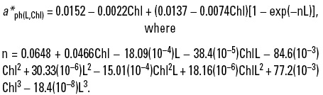
For case I waters, a*phfe chl) may be estimated with Giles-Guzmán & Álvarez-Borrego's (2000) expression:
The f-ratio (f = PNEW /PT). There are no reports on 15N incubations to estimate PNEW for the Gulf of California. Thus, it is not possible to make a direct estimate of the f-ratio for any region of the Gulf. One alternative is to use empirical algorithms developed for other regions of the world's ocean with similar hydrographic conditions to those found in the Gulf. Hidalgo-Gonzalez & Álvarez-Borrego (2004) used NO3 data from 268 hydrographic stations to generate average NO3 profiles for each season and region of the Gulf, and they used Harrison et al.'s (1987) expression (fz = fmax[1-exp(mNO3(z)/fmax)]) to calculate the f-ratio for each depth. Unfortunately, there are no reports on the fz - NO3(z) relationship for the Gulf of California. Thus, Hidalgo-Gonzalez & Álvarez-Borrego (2004) chose the parameters m and fmax as reported by Harrison et al. (1987): for the cool season they chose m = 0.98 and fmax = 0.77, which correspond to the coastal upwelling Peruvian zone; and for the warm season they chose m = 12.1 and fmax = 0.64, which correspond to the summer oligotrophic intrusion of the Southern California Bight.
DISCUSSION
Rigorous comparison of satellite-derived integrated production values for the whole euphotic zone and for the whole day (PTint) with results from 14C incubations is difficult due to the different time and spatial characteristics of these measurements (Balch & Byrne, 1994). Nevertheless, it is interesting to compare both kinds of data. Álvarez-Borrego & Lara-Lara (1991) reported 26 14C-deri-ved PTint point values for region II of the Gulf of California with an average of 1.43 g C m-2 d-1, compared with Hidalgo-Gonzalez & Álvarez-Borrego's (2004) range of 1.52-1.87 for the period 19972002; Álvarez-Borrego & Lara-Lara (1991) reported 12 point values for region III with an average of 2.1 g C m-2 d-1, compared with Hidalgo-Gonzalez & Álvarez-Borrego's (2004) range of 1.45-1.73; and Álvarez-Borrego & Lara-Lara (1991) reported four point values for region IV with a mean of 1.1 g C m-2 d-1 compared with Hidalgo-Gonzalez & Álvarez-Borrego's (2004) range of 1.52-1.68. Álvarez-Borrego & Lara-Lara (1991) only reported five point values for the warm season and for the whole Gulf, which do not allow for comparisons. In spite of great differences in time and spatial scales, both methods provided average values that are very close, and given the uncertainties of Hidalgo-Gonzalez & Álvarez-Borrego's (2004) satellite-derived estimates, these differences are not significant.
The vertical distribution of model-derived primary production is also very consistent and behaves as expected from 14C experiments. Satellite total production, PTz, presents maxima at shallower depths than those of the Chlw maxima because of greater PARz near the surface. On the other hand, PTz maxima are often in subsurface waters due to the relatively low surface Chl. With relatively high surface Chl, maximum PTz is found at the surface. The largest contribution to production is from the surface and near-surface waters (i.e., the upper 15 m), with a relatively small contribution from the DCM because of low-light levels at Zm.
Hidalgo-Gonzalez & Álvarez-Borrego (2004) performed a sensitivity analysis to assess the effect of uncertainties of variables and parameters on the estimates of average integrated total production for the whole euphotic zone and for the whole day (PTint) (g C m-2 d-1). These latter authors added and subtracted one standard error (s n-0.5) to each input variable and parameter, one at a time, to assess the effect on PTint, and they expressed the difference as percentage. When adding or subtracting one standard error to the photosynthetic parameters (P*m, α*insitu, and Φ max), it was done for all of them at the same time because they covary according to the results of Cote & Platt (1983), and Valdez-Holgufn et al. (1999). It was not possible to do a sensitivity analysis with the uncertainties associated with KPAR(z) calculated for case-I waters following Giles-Guzmán & Álvarez-Borrego (2000) because these latter authors did not provide values for the standard errors associated to their equations. However, when comparing 30 PTint values estimated with calculated PAR profiles with the corresponding values estimated with measured profiles, the mean of the percent differences was 5.9%. But, as Giles-Guzmán & Álvarez-Borrego (2000) indicated, PAR profiles that resulted from the model were smooth, whereas those that resulted from measurements in some cases had abrupt changes in the PAR vertical variation rate. Thus, possibly, most of the differences between measured and calculated PAR are caused by errors in the measured PAR values. One source of error when measuring PAR with an instrument is the optical effect of gravity waves at the sea surface; these waves focus and disperse the light very much as we can observe in a swimming pool. When lowering the instrument to measure PAR the descent is relatively fast and the instrument may catch a concentrated light beam or a dispersed one. A better way to perform the measurements would be to maintain the instrument at the same depth for few seconds, successively, each meter as it goes down, and then calculate the mean PAR for each depth, but this is usually not the way it is done. When changing K490 by one standard error, PTint changed ~2.7%. But, because of the scarce data used by Cervantes-Duarte et al. (2000) the confidence intervals of the parameters A and B are often very large, and they can yield ZPAR1% values that differ by as much as 20%. Again, more optical data are needed to better characterize case II waters.
Greatest uncertainties of the estimates for average PTint are caused by the large confidence intervals of the photosynthetic parameters. When augmenting or diminishing the photosynthetic parameters by one standard error, average PTint changed as much as 17% with low Chls, and as much as 19% with high Chls. This is because of the few degrees of freedom in the P-E parameters. The probability of having all these errors added together simultaneously is low due to the multiplication rule.
The vertical profiles of PAR can be relatively well characterized, but those of Chl need more data. Future research should focus mainly on a better characterization of the average photosynthetic parameters for each season and region within the Gulf, which are the weakest part in modeling primary production for the Gulf of California. The greatest need is for a better characterization of summer average values, both for the photosynthetic parameters and for the Chl profile.
As it was mentioned above, satellite derived estimates of PTint are in good agreement with results from 14C incubations, but there are no ship 15N data to compare with satellite derived estimates of PNEW. Hidalgo-Gonzalez & Álvarez-Borrego (2004)'s f-ratio values were particularly high for summer, up to 0.64 compared with the value suggested by Eppley (1992) of 0.1 for oligotrophic waters; but also those for winter might have been high, up to 0.77 compared to 0.4 suggested by Eppley (1992) for rich coastal waters. This is an opportunity for future research in the Gulf. 15N incubations performed in parallel with 14C incubations and nutrient determinations are needed for the whole Gulf to better characterize the parameters used in algorithms like Harrison et al.'s (1987) for the calculation of PNEW.
ACKNOWLEDGEMENTS
Francisco Javier Ponce and Jose Marfa Dominguez did the art work.
REFERENCES
Álvarez-Borrego, S. 2010. Physical, Chemical and Biological Oceanography of the Gulf of California. En: R.C. Brusca (Ed.) Gulf of California Biodiversity and Conservation. ASDM Studies in Natural History. ASDM Press and University of Arizona Press, Tucson. pp. 24-48. [ Links ]
Álvarez-Borrego, S. & G. Gaxiola-Castro. 1988. Photosynthetic parameters of northern Gulf of California phytoplankton. Continental Shelf Research 8: 37-47. [ Links ]
Álvarez-Borrego, S. & J. R. Lara-Lara. 1991. The physical environment and primary productivity of the Gulf of California. In: J.P. Dauphin and B.R. Simoneit (Eds.) The Gulf and Peninsular Province of the Californias. American Association of Petroleum Geologists. Memoir 47, Tulsa. pp. 555-567. [ Links ]
Balch, W. M. & C. F. Byrne. 1994. Factors affecting the estimate of primary production from space. Journal of Geophysical Research 99: 7555-7570. [ Links ]
Behrenfeld, M.J. & P.G. Falkowski. 1997. Photosynthetic rates derived from satellite-based chlorophyll concentration. Limnology & Oceanography 42: 1-20. [ Links ]
Behrenfeld, M. J., P. G. Falkowski, W. E. Esaias, W. Balch, J. W. Campbell, R. L. Iverson, D. A. Kiefer, A. Morel & J. A. Yoder. 1998. Toward a consensus productivity algorithm for SeaWIFS. In: Sea WLFS Technical Report Series, Vol. 42, Satellite primary productivity data and algorithm development: A Science Plan for Mission to Planet Earth, Hooker, S.B. & E.R. Firestone (Eds.), NASA/TM-1998-104566. 33 p. [ Links ]
Brusca, R. C. 2010. Introduction. In R.C. Brusca (Ed.) Gulf of California Biodiversity and Conservation. ASDM Studies in Natural History. ASDM Press and University of Arizona Press, Tucson. pp. 24-48. [ Links ]
Cervantes-Duarte, R., J. L. Mueller, C. C. Trees, H. Maske, S. Álvarez-Borrego & J. R. Lara-Lara. 2000. Euphotic depth, irradiance attenuation and remote sensing K490 in bio-optical provinces of the Gulf of California. Ciencias Marinas 26 533-560. [ Links ]
Cleveland, J. S. 1995. Regional models for phytoplankton absorption as a function of chlorophyll a concentration. Journal of Geophysical Research 100: 13,333-13,344. [ Links ]
Cortés-Lara, M. C., S. Álvarez-Borrego & A. D. Giles-Guzmán. 1999. Efecto de la mezcla vertical sobre la distribución de nutrientes y fitoplancton en dos regiones del Golfo de California, en verano. Revista de la Sociedad Mexicana de Historia Natural 49: 193-206. [ Links ]
Cote, B. & T. Platt. 1983. Day to day variations in the spring-summer photosynthetic parameters of coastal marine phytoplankton. Limnology & Oceanography 28: 320-344. [ Links ]
Ducklow, H. W., D. K. Steinberg & K. 0. Buesseler. 2001. Upper ocean carbon export and the biological pump. Oceanography 14: 50-58. [ Links ]
Dugdale, R. C. & J. J. Goering. 1967. Uptake of new and regenerated forms of nitrogen in primary productivity. Limnology & Oceanography 12: 196-206. [ Links ]
Eppley, R. W. 1992. Toward understanding the roles of phytoplankton in biogeochemical cycles: Personal notes. In P. G. Falkowski & A. D. Woodhead (Eds.) Primary productivity and biogeochemical cycles in the sea. Plenum, New York. pp. 1-7. [ Links ]
Eppley, R. W. & B. J. Peterson. 1979. Particulate organic matter flux and planktonic new production in the deep ocean. Nature 282: 677-680. [ Links ]
Falkowsky, P. G. & T. G. Owens. 1980. Light-shade adaptation: two strategies in marine phytoplankton. Plant Physiology 66: 592-595. [ Links ]
Falkowski, P. G. & J. A. Raven. 1997. Aquatic photosynthesis. Blackwell Science, Oxford. 375 p. [ Links ]
Frost, B. W. 1984. Utilization of phytoplankton production in the surface layer. In Global Ocean Flux Study: Proceedings of a Workshop, 10-14 September, 1984, Woods Hole, Massachusetts. National Academy Press, Washington, D.C., pp. 125-135. [ Links ]
Gaxiola-Castro, G., S. Álvarez-Borrego, M. F. Lavín, A. Zirino & S. Nájera-Martínez. 1999. Spatial variability of the photosynthetic parameters and biomass of the Gulf of California phytoplankton. Journal of Plankton Research 21: 231-245. [ Links ]
Giles-Guzmán, A. D. 1998. Modelos para estimar el coeficiente de atenuación vertical de luz difusa en función de la concentración de clorofila y la profundidad para aguas caso I. Tesis de Doctorado en Ciencias, División de Oceanología, CICESE, Ensenada. 93 p. [ Links ]
Giles-Guzmán, A. D. & S. Álvarez-Borrego. 1996. Covariance of the absorption of phytoplankton, colored dissolved organic matter, and detritus in case I waters, as deduced from the Coastal Zone Color Scanner bio-optical algorithm. Applied Optics 35: 2109-2113. [ Links ]
Giles-Guzmán, A. D. & S. Álvarez-Borrego. 2000. Vertical attenuation coefficient of photosynthetically active radiation as a function of chlorophyll concentration and depth in case 1 waters. Applied Optics 39: 1351-1358. [ Links ]
Gilbert, J. Y. & W. E. Allen. 1943. The phytoplankton of the Gulf of California obtained by the "E.W. Scripps" in 1939 and 1940. Journal of Marine Research 5: 89-110. [ Links ]
Gordon, H. R. & A. Morel. 1983. Remote assessment of ocean color for interpretation of satellite visible imagery: A review, Vol. 4 of Lecture Notes on Coastal and Estuarine Studies, Springer-Verlag, New York. 114 p. [ Links ]
Gordon, H. R., D. K. Clark, J. W. Brown, 0. B. Brown, R. H. Evans & W. W. Broenkow. 1983. Phytoplankton pigment concentrations in the middle Atlantic Bight: comparisons of ship determinations and CZCS estimates. Applied Optics 22: 20-36. [ Links ]
Harrison, W. G., T. Platt & M. R. Lewis. 1987. f-ratio and its relationship to ambient nitrate concentration in coastal waters. Journal of Plankton Research 9 235-248. [ Links ]
Hidalgo-González, R. M. & S. Álvarez-Borrego. 2001. Chlorophyll profiles and the water column structure in the Gulf of California. Oceanologica Acta 24: 19-28. [ Links ]
Hidalgo-González, R. M & S. Álvarez-Borrego. 2004. Total and new production in the Gulf of California estimated from ocean color data from the satellite sensor SeaWIFS. Deep-Sea Research 51: 739-752. [ Links ]
Hidalgo-González, R. M., S. Álvarez-Borrego, C. Fuentes-Yaco & T. Platt. 2005. Satellite-derived total and new phytoplankton production in the Gulf of Mexico. Indian Journal of Marine Science 34: 408-417. [ Links ]
Kirk, J. T. 0. 1993. Light and Photosynthesis in Aquatic Ecosystems. Cambridge University Press, New York. 401 p. [ Links ]
Kishino, M., M. Takahashi, N. Okami & S. Ichimura. 1985. Estimation of the spectral absorption coefficients of phytoplankton in the sea. Bulletin of Marine Science 37: 634-642. [ Links ]
Lewis, M. R., J. J. Cullen & T. Platt. 1983. Phytoplankton and thermal structure in the upper ocean: Consequences of non uniformity in chlorophyll profile. Journal of Geophysical Research 88: 2565-2570. [ Links ]
Longhurst, A., S. Sathyendranath, T. Platt & C. M. Caverhill. 1995. An estimate of global primary production in the ocean from satellite radiometer data. Journal of Plankton Research 17: 1245-1271. [ Links ]
Morel, A. & L. Prieur. 1977. Analysis of variations in ocean colour. Limnology & Oceanography 22: 709-722. [ Links ]
Morel, A. & J. F. Berthon. 1989. Surface pigment algal biomass profiles and potential production of the euphotic layer: Relationships re-investigated in view of remote sensing applications. Limnology & Oceanography 34: 1572-1586. [ Links ]
Morel, A. 1991. Light and marine photosynthesis: A model with geochemical and climatological implications. Progress in Oceanography 26: 263-306. [ Links ]
Morel, A. & S. Maritorena. 2001. Bio-optical properties of oceanic waters: a reappraisal. Journal of Geophysical Research 106: 7163-7180. [ Links ]
Petzold, T. L. 1972. Volume scattering functions for selected ocean waters. SIO Ref. 72-78, Scripps Institution of Oceanography, UCSD, La Jolla. 36 p. [ Links ]
Platt, T. & S. Sathyendranath. 1988. Oceanic primary production: Estimation by remote sensing at local and regional scales. Science 241: 1613-1620 [ Links ]
Platt, T., C. Caverhill & S. Sathyendranath. 1991. Basin-Scale estimates of oceanic primary production by remote sensing: The North Atlantic. Journal of Geophysical Research 96: 15,147-15,159. [ Links ]
Pope, R. M. 1993. Optical absorption of pure water and seawater using the integrating cavity absorption meter. Ph. D. Thesis, Texas A & M University, College Station. 243 p. [ Links ]
Preisendorfer, R. W. 1961. Application of radiative transfer theory to light measurements in the sea. Union of Geodesy and Geophysical, Institutional Monograph 10: 11-30. [ Links ]
Ryther, J. H. 1956. Photosynthesis in the ocean as a function of light intensity. Limnology & Oceanography 1: 61-70 [ Links ]
Ryther, J. H. & C. S. Yentsch. 1957. The estimation of phytoplankton production in the Ocean from chlorophyll and light data. Limnology & Oceanography 2: 281-286. [ Links ]
Santamaría-Del-Ángel, E., S. Álvarez-Borrego & F. E. Müller-Karger. 1994. Gulf of California biogeographic regions based on coastal zone color scanner imagery. Journal of Geophysical Research 99: 7411-7421. [ Links ]
Santamaría-Del-Ángel, E., S. Álvarez-Borrego, R. Millán-Nuñez & F. E. Muller-Karger. 1999. Sobre el efecto de las surgencias de verano en la biomasa fitoplanctonica del Golfo de California. Revista de la Sociedad Mexicana de Historia Natural 49: 207-212. [ Links ]
Sathyendranath, S., T. Platt, E. P. W. Horne, W. G. Harrison, 0. Ulloa, R. Outerbridge & N. Hoepffner. 1991. Estimation of new production in the ocean by compound remote sensing. Nature 353:129-133. [ Links ]
Sathyendranath, S., A. Longhurst & C. M. Caverhill. 1995. Regionally and seasonally differentiated primary production in the North Atlantic. Deep-Sea Research 42: 1773-1802. [ Links ]
Smith, E. L. 1936. Photosynthesis in relation to light and carbon dioxide. Proceedings of the National Academy of Sciences, Washington, 22: 504-511. [ Links ]
Sosik, H. M. 1996. Bio-optical modeling of primary production: consequences of variability in quantum yield and specific absorption. Marine Ecology Progress Series 143: 225-238. [ Links ]
Strickland, J. D. H. & T. R. Parsons. 1972. A Practical Handbook of Seawater Analysis. Bulletin of the Fisheries Research Board of Canada, 167 p. [ Links ]
Valdez-Holguín, J. E., S. Álvarez-Borrego & B. G. Mitchell. 1998. Photosynthetic parameters of phytoplankton in the California Current System. California Cooperative Oceanic Fisheries Investigations Reports 39: 148-158. [ Links ]
Valdez-Holguín, J. E., S. Álvarez-Borrego & C. C. Trees. 1999. Seasonal and spatial characterization of the Gulf of California phytoplankton photosynthetic parameters. Ciencias Marinas 25: 445-467. [ Links ]
Zaneveld, J. R. V., W. S. Pegau, A. H. Barnard, J. L. Mueller, H. Maske, E. Valdez, R. Lara- Lara & S. Álvarez-Borrego. 1997. Prediction of euphotic depths and diffuse attenuation coefficients from absorption profiles: a model based on comparisons between vertical profiles of spectral absorption, spectral irradiance, and PAR. Ocean Optics 14, Proceedings SPIE2963: 585-590. [ Links ]

