Artículos

 

Phytoplankton production by remote sensing in the region off Cabo Corrientes, Mexico

 

Producción fitoplanctónica por sensores remotos en la región frente a Cabo Corrientes, México

 

Daffne C. López–Sandoval¹, José Rubén Lara–Lara^2* and Saúl Álvarez–Borrego²

 

¹ Departamento de Ecología y Biología Animal, Universidad de Vigo, Ctra. Colexio Universitario s/n, Vigo, España. 36200.

² División de Oceanología, CICESE. Carretera Ensenada–Tijuana No. 3918, Zona Playitas, Ensenada, Baja California, México. 22860. *E–mail: rlara@cicese.mx

 

Recibido: 23 de junio de 2009.
Aceptado: 24 de noviembre de 2009.

 

ABSTRACT

Integrated total phytoplankton production (PP_mod) (grams of carbon per square meter per day, gC m^–2 d^–1) was calculated for the oceanic region off Cabo Corrientes, Mexico. This was done with semi–analytic models from the literature and using chlorophyll a concentrations (Chl_sat) and photosynthetically active radiation (PAR_sat) from monthly composites of the satellite sensor SeaWIFS, for May and November 2002, and June 2003. Average values for PP_mod had a seasonal variation for the inshore (1.50 and 0.70 gC m^–2 d^–1 for May and June, and 0.38 for November) and the offshore (0.55 and 0.41 gC m^–2 d^–1 for May and June, and 0.31 for November) zones. It is interesting to note that our PP_mod data are similar to the previously reported PP_14C values for the Cabo Corrientes region. In general, Chl_sat and PP_mod support the previously reported ship data, which showed intense upwelling conditions during May, an upwelling relaxation period in June, and non–upwelling in November. Estimated PP_mod values are within the range of those for other upwelling enriched ecosystems of the Pacific off Mexico.

Key words: Cabo Corrientes, upwelling, satellite chlorophyll, modeled primary productivity, Eastern Tropical Pacific.

 

RESUMEN

Se calculó la producción integrada del fitoplancton (PP_mod) (gC m^–2 d^–1) para la región oceánica frente a Cabo Corrientes, México. Se utilizaron modelos semi–analíticos publicados en la literatura científica, y concentraciones de clorofila a (Chl_sat) y la radiación fotosinteticamente activa (PAR_sat) de imágenes satelitales compuestas mensuales del sensor SeaWIFS, de mayo y noviembre 2002, y junio 2003. Los valores promedios de PP_mod tuvieron una variación estacional en la zona costera (1.50 y 0.70 gC m^–2 d^–1 para mayo y junio, y 0.38 para noviembre) y fuera de la costa (0.55 y 0.41 gC m^–2 d^–1 para mayo y junio, y 0.31 para noviembre). Los datos de PP_mod fueron similares a los valores previamente reportados de PP_14C para la región frente a Cabo Corrientes. En general, Chl_sat y PP_mod concuerdan con los datos publicados previamente, mostrando condiciones intensas de surgencias durante mayo, un periodo de relajamiento en junio y condiciones sin surgencia en noviembre. Los valores de PP_mod están dentro del rango de los reportados para otros ecosistemas del Pacífico frente a México enriquecidos por surgencias.

Palabras clave: Cabo Corrientes, surgencias, clorofila satelital, productividad primaria modelada, Pacífico Tropical oriental.

 

INTRODUCTION

Marine primary production (PP) is one of the key processes in the global carbon cycle, controlling the uptake of dissolved inorganic carbon in the euphotic zone and its transfer to the organic pool in the ocean. Through the export process the carbon is transported to the ocean's interior and eventually transported back to the surface (Schneider et al., 2007). Total production is equal to the sum of both new and regenerated production (PP = PP_new + PP_r).

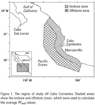
One of the main limitations of estimating PP by the traditional radiocarbon (¹⁴C) method is the small number of point samples generated for a particular area, and the poor temporal coverage. Thus, satellite ocean color offers an alternative to estimate the phytoplankton primary production rates in the oceans with an ample spatial–temporal variability that is not possible to cover by research vessels. The early models for primary production estimation in the ocean were based on laboratory experiments to characterize the light–chlorophyll relationship (Ryther, 1956). They offered the basis for models that make use of variables measured from remote sensors (e.g., pigments, irradiance, etc.) (Longhurst et al., 1995; Hidalgo–González et al., 2005). It has been argued that instantaneous point PP values based on satellite data are very imprecise, but when the average of satellite data are used for whole oceanic regions, and for relatively large time scales, such as months or seasons, the estimated PP values can adequately represent very well the biological dynamics of those regions (Hidalgo–González & Álvarez–Borrego, 2004). The large number (n) of pixels within our region of interest (Fig. 1), and for whole months, allows for very precise pigment (Chl_sat) and PAR_sat (Photosynthetic Active Radiation) averages with relatively small standard errors (s/n^0.5).

Remote sensors provide information on the photosynthetic pigment concentration for the upper 22% of the euphotic zone (Kirk, 1994). To model primary production in the water column from satellite–derived photosynthetic pigments, estimates of the vertical distribution of pigment concentration are required, whereas the assumption of a mixed layer with a homogeneous pigment distribution could lead to inaccurate estimates of integrated primary production (Platt et al., 1991). The deep chlorophyll maximum (DCM) is a consistent feature in the ocean (Cullen & Eppley, 1981). Generally, accounting for its presence increases estimates of integrated production.

Radiocarbon primary production data (PP_14C) for the area off Cabo Corrientes covering the whole spectrum from oligotrophic to eutrophic waters (from 0.17 up to 1.40 gC m^–2 day^–1), are very scarce (Zeitzschel, 1969; Gaxiola–Castro & Álvarez–Borrego, 1986; Lara–Lara & Bazán–Guzmán, 2005). López–Sandoval et al. (2009) applied the ¹⁴C method to study the spatial and temporal variation of PP_14C in this region for May and November 2002, and June 2003. However, due to the poor spatial resolution of this method, to the very few generated data, and to the ample hydrographic variability of the zone, we decided to estimate average values of PP using remote sensing based models (PP_mod), and to make comparisons with average PP_14C values for the same months and areas within our region of interest. Our objective was to obtain representative average primary production values for whole months and zones within the region off Cabo Corrientes, in contrast to few instantaneous point ¹⁴C estimates.

 

MATERIALS AND METHODS

The study region off Cabo Corrientes, is located between 18° and 22° N, and from 104° 10' to 107° 25' W (Fig. 1). This is the region covered by the three oceanographic cruises of López–Sandoval et al. (2009) (locations of hydro–stations are shown in figure 2). A line joining Cabo San Lucas and Cabo Corrientes defines the entrance to the Gulf of California. Thus, the northern part of our study area is at the southeastern portion of the entrance to the gulf. Winds are from the northwest for most of the year, with maximum speeds during winter and spring, and from the southeast during summer and autumn. The region has been characterized by the presence of mesoscale structures such as eddies, thermal fronts, and coastal upwelling events (Lavín et al., 2006; Zamudio et al., 2007). Upwelling conditions in this region may result with alongshore winds during winter and spring (Roden, 1972); and also as a result of the interaction between coastal currents and the physiography, mainly Cabo Corrientes, similar to the generation of cold–water plumes off Point Conception, California, as described by Fiedler (1984). Coastal upwelling has an important effect on the nutrient supply to the euphotic zone and hence on chlorophyll a concentrations (Chl mg m^–3) and PP. The geostrophic currents are equatorward during winter and spring off Cabo Corrientes (thus propitious to upwelling), while during summer and autumn they are poleward (figure 7 in Keesler, 2006). This causes downwelling near the coast, and the sinking of the thermocline, with oligotro–phic waters at the surface during summer and autumn.

To generate the PP vertical profiles (mgC m^–3 h^–1, with a PP_z value for each meter), we used the model proposed by Platt et al. (1991), and the modification proposed by Hidalgo–González and Álvarez–Borrego (2004). Platt et al.'s (1991) model is a non–homogenous, non–spectral model, and this means that Chl is allowed to change with depth (Chl_z) by means of a Gaussian curve that reproduces the DCM, but the change of the spectral distribution of PAR with depth is not taken into consideration. Hidalgo–González and Álvarez–Borrego's (2004) modification is a non–homogeneous, spectral model that allows for the change of the spectral distribution of irradiance with depth, based on the method proposed by Giles–Guzmán and Álvarez–Borrego (2000). To estimate PP_mod (mgC m^–2 d¹), the region off Cabo Corrientes was separated into an inshore zone (< 60 km from the coast) and an offshore zone (> 60 km; Fig. 1) following López–Sandoval (2007). PP_z was generated for each hour from dawn to dusk, with a variable PAR_z for different hours of the day, and a constant Chl_z with time. Each PP_z profile was integrated with depth from z = 0 to the bottom of the euphotic zone (Z_eu) to transform from mgC m^–3 h^–1 to mgC m^–2 h^–1 (PP_int = ΣPP_z, where z changes meter by meter). Z_eu was considered to be the depth where PAR_z = 0.01(PAR_o). Then PP_int values were integrated for the whole day to calculate PP_mod = SPP_int, with a PP_int value for each hour of the day (to transform from mgC m^–2 h^–1 to gC m^–2 d¹). Finally, to estimate PPn_ew f–ratio values (PP_new/PP_mod) of 0.4 and 0.1 were applied to the PP_mod values of the inshore and offshore zones, respectively, following Eppley's (1992) suggestion.

We used Platt et al.'s (1991) model for the inshore zone data of May 2002, which had case II waters (Chl>1.5 mg m^–3):

PP_z = [P*_mChl_sat(z) α*_PAR PAR_z] x [(P*_m)² + (PAR_z α*_PAR)²]^–0.5 mgC m^–3 h^–1,

where: the asterisk means that the value is normalized per unit of chlorophyll concentration; P*_m (mgC (mg Chl)^–1 h^–1) is the photosynthetic rate at optimum irradiance; Chl_sat(z) is the average Chl for depth z for the chosen oceanic zone (inshore or offshore), derived from the monthly satellite composite and a model for the Chl vertical distribution; α*_PAR (mgC (mg Chl)^–1 h^–1 (μmol quanta m^–2 s^–1 )1) is the initial slope of the photosynthesis–irradiance (P–E) curve; and PAR is the scalar photosynthetically active radiation (400–700 nm, μmol quanta m^–2 s^–1 ). The photosynthetic parameters, P*_m and α*PAR, are derived from photosynthesis–irradiance (P–E) experiments in such a way that, in combination with Chl, they represent the whole photosynthetic capacity of phyto–plankton, and there is no need to include the concentration of other pigments. The implicit assumption is that, although phyto–plankton populations can vary in their composition, their suite of pigments does not change in such a way as to make a significant impact on photosynthetic rates.

Hidalgo–González and Alvarez–Borrego's (2004) modification was used in those cases when the chlorophyll profiles showed case I waters (Chl < 1.5 mg m^–3). These waters correspond to the offshore zone of May 2002, and of both inshore and offshore zones of November 2002 and June 2003:

PP_z = [P*Φ_max Chl_sat(z) a*_ph(z, _chl) PAR_z× [(0.02315P*_m)²+ (PAR_zΦ_max a*_ph(z,chl))²]^–0.5 mgC m^–3 h^–1.

In this equation Φ_max is the maximum quantum yield (mol C (mol quanta)^–1), and a*_ph(z,chl) (m² (mg Chl)^–1) is the phytoplankton specific absorption coefficient of light averaged for the spectral distribution of PAR at depth. This corrects the initial slope α*PAR for the spectral distribution of the in situ scalar PAR. In place of α^*_PAR the product 43.2Φ_max a*_ph(z,chl) was used (Giles–Guzmán & Álvarez–Borrego, 2000). The factor 43.2 converts mol C to mgC, seconds to hours, and mol quanta to μmol quanta. These expressions show that in order to estimate PP_z not only the surface Chl value is needed, but also the vertical profiles of Chl and PAR.

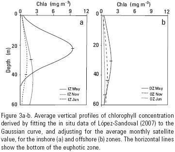
Surface chlorophyll (Chl_sat) and PAR (PAR_sat) monthly composites were taken from the SeaWIFS sensor (Sea–viewing Wide Field–of–view Sensor) archive data (http://oceancolor.gsfc.nasa.gov/). These are Chl_sat maps produced with the standard algorithm of the GSFC (Goddard Space Flight Center), with a 9 km² resolution. No filter was used to smooth the original data. An average Chl_sat was taken from the monthly satellite composites, for each zone within our region. For the application of both production models, an average chlorophyll profile was estimated for each month and zone (inshore and offshore) from the ship Chl_(z) data in López–Sandoval (2007) and it was adjusted to the respective average Chl_sat. Following Platt et al. (1988), a Gaussian distribution function was fitted to the ship Chl_(z) data from each hydro–station. The Gaussian equation is:

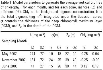
Chl_z = Chl_o + [h/σ(2π)^0.5]exp[–(Z – Z_m)²/2σ²],

where Chl_z is the chlorophyll concentration (mg m^–3) at depth Z (m), Chl_o is the background pigment concentration, h is the total pigment (mg m^–2) above the baseline Chl_o (h is the area under the Gaussian curve and it is larger than the integrated Chl for the euphotic zone, Chl_int), σ controls the thickness of the DCM layer, and Z_m is the depth of the DCM. For each month and zone, average values of the parameters Chl_o, h, σ, and Z_m were calculated to generate a single Chl profile (table 1). Then, each average chlorophyll profile was adjusted so the surface had the average value from the satellite monthly composite. To do this, Z_m was adjusted following Hidalgo–González and Álvarez–Borrego (2008). Through this adjustment Chl_z was transformed to Chl_sat(z). Two deep Chl maxima were reported for the three cruises, one between 20 and 50 m, and a second generally deeper than 90 m (López–Sandoval, 2007). Due to the very low values of PAR_z (<1% of PAR_o) for depths greater than 70 m, estimates of PP_z for the second maximum indicate that its contribution to the integrated value (PP_mod) is not significant. Thus, for the purpose of fitting the ship data to the Gaussian curve, the second deeper Chl maximum was not considered.

Average PAR_sat values were taken from the monthly satellite composites for our study region, for each of the three studied months. The SeaWIFS algorithm provides PAR_sat values corresponding to z = 0 (just below the sea–surface). These are daily average values (mol quanta m^–2 d¹). The shape of the diurnal variation of incident irradiance illustrated by Kirk (1994) was used to adjust these PAR_sat values to obtain average PAR_o, _t values (μmol quanta m^–2 s¹) for each hour from dawn to dusk. This implies the assumption of uniform cloudiness throughout the average day. Sets of PAR_z, _t profiles were generated for each zone and month from these PAR_o, _t values following Giles–Guzmán and Álvarez–Borrego's (2000) method for case I waters. This method is based on the Lambert–Beer law (PAR_z, _t = PAR_o, _t exp(–K_zZ). This law was applied meter–by–meter allowing for the spectral change of irradiance with depth and its effect on a variable K_z. When Chl_z values >1.5 mg m^–3 were found near and at the DCM, the PAR_z, _t values were calculated following Giles–Guzmán and Álvarez–Borrego's (2000) method for the surface and subsurface water layers (with Chl_z <1.5 mg m^–3), and a constant K_z (equal to the one for Chl_z = 1.5 mg m^–3) was used for the deep layer (with Chl_z >1.5 mg m^–3).

There are no data on the photosynthetic parameters of phytoplankton for this oceanic region. Thus, as a first approximation, we used the average values proposed by Cullen (1990) for these parameters: P*_m = 4.8 mg C (mg Chl)^–1 h^–1 and α*_PAR(z) = 0.017 (mgC (mg Chl)^–1 h^–1 (µmol quanta m^–2 s^–1 )^–1). The phytoplankton specific absorption coefficient (α*_ph(z,ch) (m² (mg Chl)^–1) was calculated following Giles–Guzmán and Álvarez–Borrego (2000).

 

RESULTS

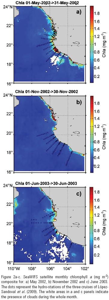
Average PAR_o, _t values for noon were 1670, 965, and 1490 ujmol quanta m^–2 s^–1 for May and November 2002, and June 2003, respectively (Fig. 2a–c). The largest average depth of the euphotic zone (Z_eu) was 54 m and it was for the offshore zone of June 2003 while the smallest Z_eu was 22 m for the inshore zone of May 2002. The May Chl_sat distribution showed relatively high values south of Cabo Corrientes, with highest values in the inshore zone (Fig. 2a). The June 2003 Chl_sat distribution also showed relatively high values in the inshore zone, but with a much smaller spatial coverage than that of the May composite (Fig. 2c). The November Chl_sat distribution showed in general very low values, with few exceptions in the inshore zone north of Cabo Corrientes, outside the region covered by the oceanographic cruises of López–Sandoval et al. (2009; Fig. 2b). The monthly mean Chl_sat for May 2002 was 0.60 and 0.47 mg m^–3 for the inshore and the offshore zones, respectively; for November 2002 it was 0.42 and 0.17 mg m^–3 for the inshore and the offshore zones, respectively; and for June 2003 it was 0.27 mg m^–3 for both zones.

The average modeled chlorophyll profile for the inshore zone of May 2002 had the largest Chl_z values of all zones and months (Fig. 3a). Its maximum was ~9.4 mg m^–3 and it was at the bottom of the euphotic zone. The average Chl_z profile with the lowest values was the one for the offshore zone of June 2003, with a Chl maximum of 0.58 mg m^–3 at 44 m, 10 m above the bottom of the euphotic zone (not visually appreciable in figure 3b). The euphotic zone integrated modeled chlorophyll (Chl_int) had maximum average values for May, for both, inshore (116.6 mg m^–2) and offshore (38.9 mg m^–2) zones. November 2002 had intermediate Chl_int average values with 41.4 and 30.7 mg m^–2 for the inshore and offshore zones, respectively. June 2003 presented the lowest Chl_int average values with 33.1 and 25.9 mg m^–2, for the inshore and offshore zones, respectively.

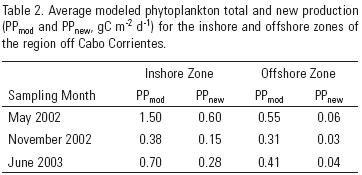
Average PP_mod for the inshore zone of May 2002 was much larger (1.50 gC m^–2 d^–1) than that for the offshore zone (0.55 gC m^–2 d^–1). Average PP_mod for both inshore and offshore zones of November 2002 were close to each other (0.38 and 0.31 gC m^–2 d^–1, respectively). Average PP_mod values for June 2003 showed a clear gradient with a higher inshore value than that of the offshore zone, 0.70 and 0.41 gC m^–2 d^–1, respectively (table 2). In accordance with the PP_mod values, average PP_new value for the inshore zone of May 2002 (0.60 gC m^–2 d^–1) was larger than the inshore value for June 2003, and this was higher than the one for November 2002; and a similar temporal change resulted for the offshore zone (table 2).

 

DISCUSSION

Phytoplankton production calculated from remote sensed data on ocean color, which depend on parameters developed from ship observations, yield more representative estimates of the large–scale average production than those calculated from ship data alone (Platt et al., 1991). Morel and Berthon (1989) indicated that it is unreasonable and probably superfluous to envisage the use of a light–production model on a pixel–by–pixel basis when interpreting satellite imagery. Our objective was to obtain representative average production values for whole months and zones within the region off Cabo Corrientes.

The vertical resolution of the Chl_sat(z) profiles offer significant advantages when compared to models that use homogeneous Chl_sat profiles, because they take into account the phytoplankton biomass and the light field vertical variability throughout the water column. Based on the hydrography, López–Sandoval (2007) defined the two zones within the Cabo Corrientes region, inshore and offshore.

López–Sandoval et al. (2009) reported that the upwelling index shows the beginning of the upwelling period in January, it is relatively intense from March through May, relaxing in June, and with a non–upwelling period from July through December. López–Sandoval et al. (2009) also reported low values of sea surface temperature (SST) and high Chl near the coast with uplifting of the thermocline towards the coast for May 2002 and June 2003. During May and June, the enrichment of the coastal zone seems to be the result of nutrient inputs from below the euphotic zone as a result of upwelling. This was in spite of a moderate El Niño reported for the years 2002 and 2003 (Durazo et al., 2005). This event was detected in March 2002 for the area between 5° S and 5° N. El Niño events arrive about half a year later to the entrance region of the Gulf of California (Robles–Pacheco & Christensen, 1983). Thus, our May 2002 data were collected previous to the arrival of this El Niño. A thorough analysis of data on sea surface temperature and sea–level anomalies would be necessary to find out if the effect of this El Niño was significant for our June 2003. This migth explain the relatively low values of Chl_sat obtained for this month. Nevertheless, as it was mentioned above, there is evidence of upwelling in our study area during June 2003.

In general, the parameters that were used in this study to model the vertical chlorophyll profile could be considered as representatives of the two zones and the three periods that characterize the region. However, more ship Chl data are needed to better characterize the means of the Gaussian parameters and their temporal and spatial variation.

Rigorous comparison of satellite–derived PP_mod values with average results from ¹⁴C incubations is difficult due to the very different time and space characteristics of these measurements (Hidalgo–González & Álvarez–Borrego, 2004). Nevertheless, it is interesting to compare both kinds of data. Our PP_mod average values largely overestimated (they are two or threefold) the PP_14C average values from López–Sandoval et al. (2009) for both inshore and offshore zones. López–Sandoval et al.'s (2009) PP_14C data are very few and very scattered, with a large standard error (up to 88% of the mean). However, in agreement with the PP_14C results reported by López–Sandoval et al. (2009), our PP_mod values were highest for May (within the relatively intense upwelling season), they were followed by those for June (during the upwelling relaxation period), and they were lowest for November when stratification was strongest.

Gaxiola–Castro and Álvarez–Borrego (1986) reported two point instantaneous PP_14C values for January (within the upwe–lling season) and for the offshore zone off Cabo Corrientes (0.41 and 1.40 gC m^–2 d_–1), and Lara–Lara and Bazán–Guzmán (2005) reported 0.17 and 0.42 gC m^–2 day^–1 also for January, compared to our PP_mod average value of 0.55 gC m^–2 day^–1 for May 2002. On the other hand, Zeitzschel (1969) reported a single instantaneous point estimate for our offshore zone and for November (0.45 gC m^–2 day^–1), which is 45% larger than our PP_mod average value for that month. Thus, these PP_14C data suggest that phytoplankton production is very patchy in this region of the ocean and that our PP_mod average values may be much more representative than instantaneous point estimates.

Possibly, part of the differences between PP_mod and PP_14C were due to the use of constant values for the photosynthetic parameters in a region of ample spatial and temporal environmental variability. The effect of nutrient concentration is not explicit in our primary production models because it is implicit in the Chl values. Nutrients control phytoplankton biomass but have a very weak effect on photosynthetic parameters (Cullen et al., 1992). It has long been known that photosynthetic parameters change with depth and time (Falkowski & Owens, 1980; Valdéz–Holguín et al., 1999). Also, Montecino et al. (2004) have shown that there are significant variations of the photosynthetic parameters during upwelling events; usually they have lower values during the intense phase of upwelling than during the relaxation period. Tonn et al. (2000) also reported lower values for the photosynthe–tic parameters in the upwelling area of the Arabic Sea than those for the surroundings. Conditioning to a higher irradiance regime could produce higher photosynthetic parameters (Falkowski & Owens, 1980). When upwelling is intense phytoplankton is conditioned to a lower irradiance regime, because water is arriving at the euphotic zone from below, and when upwelling relaxes or there is strong stratification phytoplankton cells at or near the sea surface are conditioned to a higher irradiance regime. Data on time and space variation of photosynthesis–irradiance (P–E) parameters are needed for this region off Cabo Corrientes.

The submarine light field (PARz) is very well characterized by the methodology reported by Giles–Guzmán & Alvarez–Borrego (2000). In spite of possible errors, ocean color satellite imagery are very consistent; the seasonal cycles and the spatial variation of Chl_sat behave very much as expected according to physical phenomena such as currents, eddies and the occurrence of upwelling (Hidalgo–González & Álvarez–Borrego, 2004). Trees et al. (2000) reported that, despite the various sampling periods and numerous geographic locations, there are consistent patterns in the ratios of the log accessory pigments to log total Chl (Chl a, Chl a allomer, Chl a epimer, and chlorophyllide a), and there is a strong log–linear relationship for these ratios. Trees et al. (2000) indicated that this log–linearity largely explains the success in remotely sensed chlorophyll algorithms, even though phytoplankton populations can vary in their composition and suite of pigments. Thus, most of the uncertainties of PP_mod values for this region of the ocean are mainly due to the lack of proper knowledge on the variations of the photosynthetic parameters (P^*_m and α^*_PAR, and quantum efficiency derived from the latter as shown above). Nevertheless, even with average photosyn–thetic parameters as those used in this work, a reasonable first approximation to the biological dynamics of this region has been attained. The seasonal and spatial variations of PP have been described in a similar fashion as that using the ¹⁴C method, but with a greater spatial and temporal coverage.

Pennington et al. (2006) used satellite ocean color images to show that during spring this region off Cabo Corrientes develops high pigment concentrations, and this is mainly due to coastal upwelling events. On the other hand, during late autumn (November) the lowest Chl and PP_mod were registered. This was probably due to downwelling causing a deeper and stronger thermocline. This caused the inshore and offshore zones to exhibit similar PP_mod values due to very oligotrophic coastal waters. The vertical salinity distribution reported by López–Sandoval (2007) clearly show the low surface values inshore indicating the presence of the Surface Equatorial Water Mass, with warm and low nutrient waters. A factor causing part of the decline in PP_mod for November 2002 was the relatively low PAR_o average value, 965 μmol quanta m^–2 s^–1 compared to 1670 for May 2002. This caused ~14% of the difference between the PP_mod estimates for these two months, the rest of the difference was caused by the larger Chl_sat(z) values for May. The relatively low PAR_o November values were due to the seasonal cycle of irradiance and the relatively large cloud coverage during this month.

The spring PP_mod values for our study area were of similar magnitude as the values reported for other productive regions off the Mexican Pacific coast. For example, Alvarez–Borrego and Lara–Lara (1991) reported 26 PP_14C data for "winter" conditions of the central Gulf of California with an average of 1.43 gC m^–2 d^–1. They reported 12 values for the big islands region of the gulf with an average of 2.1 gC m^–2 d^–1 , and four values for the northern gulf with an average of 1.1 gC m^–2 d^–1,compared to our May value of 1.50 gC m^–2 d^–1 for the inshore zone. Also, our spring inshore PP_mod rates are comparable to the PP_14C data reported by Gaxiola–Castro and Álvarez –Borrego (1986) for the entrance to the Gulf of California (for January, from 0.19 to 1.40 gC m^–2 d^–1), and to the satellite–derived values reported by Hidalgo–González and Álvarez–Borrego (2004) for the upwelling season of the Gulf of California (1.16 – 1.91 gC m^–2 d^–1).

Our PP_new values for the inshore zone are between half and ~150% of the values reported by Hidalgo–González and Álvarez–Borrego (2004) for the entrance region of the Gulf of California. The value for May 2002 is between ~45% and ~85% of those reported by these latter authors for the upwelling season of the middle and northern Gulf of California.

The description of the temporal and spatial variability of PP_new may give us an idea of the variability of the flux of organic matter out of the surface layer. Since the organic matter is degraded in its way down to the bottom and only the most refractive particles reach the bottom, e–ratio values (the fraction of PP reaching the bottom) are expected to be smaller than f–ratios. Organic particle flux has not been measured in our region of interest. Therefore, data needs to be generated on this issue for a clear understanding of its benthic ecological dynamics. In any case, the PP_new seasonality in the region off Cabo Corrientes shows that this flux of organic matter is much lower during summer and autumn than during the upwelling season.

Our data show that the region off Cabo Corrientes exhibits significant seasonality in the PP_mod rates. In general, seasonal cycles are weak over much of the open–ocean eastern tropical Pacific, but several eutrophic coastal areas do exhibit substantial seasonality (Pennington et al., 2006). Our results corroborate it. Undoubtedly, this is a response to the physical and chemical environmental variability of the study area. This was caused by upwelling that enhances the rates of nutrient supply to maintain high levels of primary production, much above those of oligotrophic waters.

 

ACKNOWLEDGMENTS

This work was supported by CONACYT (Mexico) through contract SEP–2004–C01–45813/A1, and through a scholarship for the first author. It was also supported by CICESE. J.M. Dominguez and F.J. Ponce did the art graphics.

 

REFERENCES

Alvarez–Borrego, S. & J. R. Lara–Lara. 1991. The physical environment and primary productivity of the Gulf of California. In: J. P. Dauphin & B. Simoneit (Eds.): The gulf and peninsular province of the Californias. Monographs of the American Association of Petroleum Geologists 47: 555–567.        [ Links ]

Cullen, J. J. 1990. On models of growth and photosynthesis in phytoplankton. Deep–Sea Research 37: 667–683.        [ Links ]

Cullen, J. J. & R. W. Eppley. 1981. Chlorophyll maximum layers of the Southern California Bight and possible mechanisms of their formation and maintenance. Oceanologica Acta 4: 23–32.        [ Links ]

Cullen, J. J., X. Yang & H. L. Macintyre. 1992. Nutrient limitation and marine photosynthesis. In: P.G. Falkowski & A.D. Woodhead (Eds.). Primary productivity and biogeochemical cycles in the sea. Plenum, New York, 550 p.        [ Links ]

Dugdale, R. C. & J. J. Goering. 1967. Uptake of new and regenerated forms of nitrogen in primary productivity. Limnology and Oceanography 12: 196–206.        [ Links ]

Durazo, R., G. Gaxiola–Castro, B. Lavaniegos, R. Castro–Valdez, J. Gómez–Valdés, & A. Da S. Mascarenhas Jr. 2005. Oceanographic conditions west of the Baja California coast, 2002–2003: A peak El Niño and subarctic water enhancement. Ciencias Marinas 31: 537–552.        [ Links ]

Eppley, R. W. 1992. Toward understanding the roles of phytoplankton in biogeochemical cycles: Personal notes. In: P.G. Falkowski & A.D. Woodhead (Eds.). Primary productivity and biogeochemical cycles in the sea, Plenum, New York, 550 p.        [ Links ]

Eppley, R. W. & B. J. Peterson. 1979. Particulate organic matter flux and planktonic new production in the deep ocean. Nature 282: 677–680.        [ Links ]

Falkowski, P. G. & T. G. Owens. 1980. Light–shade adaptation: two strategies in marine phytoplankton. Plant Physiology 66: 592–595.        [ Links ]

Fiedler, P. C. 1984. Satellite observations of the 1982–1983 El Niño along the U.S. Pacific coast. Science 224: 1251–1254.        [ Links ]

Gaxiola–Castro, G. & S. Álvarez–Borrego. 1986. Primary productivity of the Mexican Pacific. Ciencias Marinas 12: 26–33.        [ Links ]

Giles–Guzmán, A. D. & S. Álvarez–Borrego. 2000. Vertical attenuation coefficient of photosynthetically active radiation as a function of chlorophyll concentration and depth in case 1 waters. Applied Optics 39: 1351–1358.        [ Links ]

Hidalgo–González, R. M. & S. Álvarez–Borrego. 2004. Total and new production in the Gulf of California estimated from ocean color data from the satellite sensor SeaWIFS. Deep–Sea Research II 51: 739–752.        [ Links ]

Hidalgo–González, R. M. & S. Álvarez–Borrego. 2008. Water column structure and phytoplankton biomass profiles in the Gulf of Mexico. Ciencias Marinas 34: 197–212.        [ Links ]

Hidalgo–González, R. M., S. Álvarez–Borrego, C. Fuentes–Yaco & T. Platt. 2005. Satellite–derived total and new phytoplankton production in the Gulf of Mexico. Indian Journal of Marine Sciences 34: 408–417.        [ Links ]

Kessler, W.S. 2006. The circulation of the eastern tropical Pacific: A review. Progress in Oceanography 69: 181–217.        [ Links ]

Kirk, J. T. O. 1994. Light and photosynthesis in aquatic ecosystems. Cambridge University Press, New York, 509 p.        [ Links ]

Lara–Lara, J. R. & C. Bazán–Guzmán. 2005. Distribución de clorofila y producción primaria por clases de tamaño en la costa del Pacífico mexicano. Ciencias Marinas 31: 11–21        [ Links ]

Lavín, M. F., E. Beier, J. Goméz–Valdés, V. M. Godínez & J. García. 2006. On the summer poleward coastal current off SW México. Geophysical Research Letters 33: L02601, doi:02610.01029/02005GL024686.        [ Links ]

Longhurst, A., S. Sathyendranath, T. Platt, & C. M. Caverhill. 1995. An estimate of global primary production in the ocean from satellite radiometer data. Journal of Plankton Research 17: 1245–1271.        [ Links ]

López–Sandoval, D. C. 2007. Variabilidad de la productividad primaria en la región de Cabo Corrientes, México. Tesis de Maestría en Ciencias, Centro de Investigación Científica y de Educación Superior de Ensenada, B.C. Ensenada, 69 p.        [ Links ]

López–Sandoval, D. C., J. R. Lara–Lara, M. Lavín, S. Álvarez–Borrego & G. Gaxiola–Castro. 2009. Primary productivity in the Eastern Tropical Pacific off Cabo Corrientes, Mexico. Ciencias Marinas 35: 169–182.        [ Links ]

Montecino, V., R. Astoreca, G. Alarcón, L. Retamal & G. Pizarro. 2004. Bio–optical characteristics and primary productivity during upwelling and non–upwelling conditions in a highly productive coastal ecosystem off central Chile (~36ºS). Deep–Sea Research II 51: 2413–2426.        [ Links ]

Morel, A. & J. F. Berthon. 1989. Surface pigment algal biomass profiles and potential production of the euphotic layer: Relationships rein–vestigated in view of remote sensing applications. Limnology and Oceanography 34: 1572–1586.        [ Links ]

Pennington, T. J., K. L. Mahoney, V. S. Kuwahara, D. D. Kolber, R. Calienes & F. P. Chavez. 2006. Primary Production in the eastern tropical Pacific: A review. Progress in Oceanography 69: 285–317.        [ Links ]

Platt, T., C. Caverhill & S. Sathyendranath. 1991. Basin–Scale estimates of oceanic primary production by remote sensing: The North Atlantic. Journal of Geophysical Research 96: 15,147–15,159.        [ Links ]

Platt, T., S. Sathyendranath, C. M. Caverhill & M. R. Lewis. 1988. Ocean primary production and available light: further algorithms for remote sensing. Deep–Sea Research I 35: 855–879.        [ Links ]

Robles–Pacheco, J. M., & N. Christensen. 1983. Effects of the 1982–83 El Niño on the Gulf of California. EOS Transactions 64: 103.        [ Links ]

Roden, G. 1972. Termohaline structure and baroclinic flow across the Gulf of California entrance and in the Revillagigedo Islands region. Journal of Physical Oceanography 2: 177–183.        [ Links ]

Ryther, J. H. 1956. Photosynthesis in the ocean as a function of light intensity. Limnology and Oceanography 1: 61–70        [ Links ]

Schneider, B., L. Boop, M. Gehlen, J. Segschneider, T. l. Frolicher, F. Joos, P. Cadule, P. Friedlingstein, S. C. Doney & M. J. Behrenfeid. 2007. Spatio–temporal variability of marine primary and export production in three global coupled climate carbon cycle models. Biogeosciences Discuss 4: 1877–1921.        [ Links ]

Toon, R. K., S. E. Lohrenz, C. E. Rathbun, A. M. Wood, R. A. Arnone, B. H. Jones, J. C. Kindle & A. D. Widemann. 2000. Photosynthesis–irradiance and community structure associated with coastal filaments and adjacent waters in the northern Arabian Sea. Deep–Sea Research II 47: 1249–1277.        [ Links ]

Trees, C. C., D. K. Clark, R. R. Bidigare, M. E. Ondrusek & J. L. Muller. 2000. Accessory pigments versus Chlorophyll a concentrations within the euphotic zone: A ubiquitous relationship. Limnology and Oceanography 45: 1130–1143.        [ Links ]

Valdéz–Holguín, J. E., S. Álvarez–Borrego & C. C. Trees. 1999. Seasonal and spatial characterization of the Gulf of California phytoplankton photosynthetic parameters. Ciencias Marinas 25: 445–467.        [ Links ]

Zamudio, L., H. E. Hurlburt, J. E. Metzger & C. E. Tilburg. 2007. Tropical wave–induced oceanic eddies at Cabo Corrientes and the María Islands, México. Journal of Geophysical Research 112(C05048), doi:10.1029/2006jc004018.        [ Links ]

Zeitzschel, B. 1969. Primary productivity in the Gulf of California. Marine Biology 3: 201–207.        [ Links ]