Matemáticas y ciencias sociales

 

Abstract Labour in a Model of Joint Production*

 

Takao Fujimoto** Fumiko Ekuni***

 

** Fukuoka University, Fukuoka, Japan. Correo electrónico: takao@econ.fukuoka–u.ac.jp.

*** Shikoku–Gakuin University, Zentsuji, Japan. Correo electrónico: fumiko@sg–u.ac.jp.

 

Artículo recibido el 12–04–10
Artículo aceptado el 10–11–10

 

Abstract

This paper presents a new mathematical method for constructing abstract labour as conceived by Karl Marx, in a general input–output model with joint production and heterogeneous labour. A brief history of previous efforts to define and compose abstract labour using input–output models is also described. A numerical example is given to show how our method works in a concrete way.

Key words: abstract labour, eigenvalue, eigenvector, heterogeneous labour, Kakutani fixed point theorem.

 

Resumen

Este artículo presenta un nuevo método matemático para construir el trabajo abstracto concebido por Karl Marx, mediante un modelo de insumo–producto con el trabajo heterogéneo y la producción conjunta. También se describe una historia breve sobre los esfuerzos para definir y componer una abstracción matemática usando los modelos de entrada–salida. Se dan una serie de ejemplos numéricos que nos muestran cómo funciona el método de manera concreta.

Palabras clave: trabajo abstracto, valor propio, vector propio, trabajo heterogéneo, teorema de punto fijo de Kakutani.

 

1. INTRODUCCION

Productivity can be enhanced by introducing division of labour. This fact has been well known, and we believe that in reality division of labour has played a significant role in the development of human societies. Yet, theoretical analysis of heterogeneity of labour has been given little attention by economists. When heterogeneity of labour is allowed for in a model of economy, some basic problems emerge. The first problem is concerned with how to measure labour values of various commodities and labour services. The second one is whether we could devise abstract labour, using given technological data. The third may be how to define rates of exploitation for individual types of labour services and for abstract labour. Some economists regard the reduction of heterogeneous labour to abstract labour as unnecessary, while others think of the reduction as essential to theory of exploitation.

Surely, it may sometimes be necessary to know the rate of exploitation for the working class as a whole, in addition to the rates for individual types of labour. Then, it becomes indispensable to carry out the reduction of various types of labour to a common unit or abstract labour. Besides, it may be interesting to study how to realize the uniform rate of exploitation among heterogeneous groups of labour if at all the reduction is performed.

This paper represents a way of finding out reduction ratios, in a general model with joint production and heterogeneous labour, by use of linear programming problems and Kakutani fixed point theorem. Our method guarantees the uniform rate of exploitation among all the types of labour. In section 2, we include a brief history of the researches on the topic. Section 3 explains our model and how it is more general than the existing ones. Section 4 describes our method for somewhat restrictive cases. Section 5 presents a numerical example to show how our method works. Then section 6 describes our approach to a still more general model where each household activity can produce a plural number of labour services jointly and some labour services are produced by normal production processes. Final section 7 includes some concluding remarks. It should be noted at the outset that we deal only with mathematical aspects of abstract labour, and do not touch upon historical and philosophical sides of the topic. We hope that this article will stimulate discussions among those philosophers and historians who are interested in abstract labour.

 

2. BRIEF HISTORY

While Marx (1865) stressed the heterogeneity of human labour when he considered the values of various labour services and their prices, Marx (1867) shifted the focus to abstract labour or "human labour in the abstract" in order to unite heterogeneous labour into one working class.¹ He wrote: "Skilled labour counts only as simple labour intensified, or rather, as multiplied simple labour, a given quantity of skilled being considered equal to a greater quantity of simple labour [...] For simplicity's sake we shall henceforth account every kind of labour to be unskilled, simple labour".² Thus, Marx did not explain how to derive reduction ratios.

As early as in 1913, Potron (1913) used a model with heterogeneous labour without joint production.³ Potron's paper attracted little attention in his days, while Bowles–Gintis's (1977), 65 years after Potron, was the starter of a series of more recent research efforts thereafter for a short period.⁴ Most of contributions dealt with models without joint production, and two notable exceptions are Steedman (1980) and Krause (1980).⁵ Steedman (1980) insists that there is no need to reduce heterogeneous labour to abstract labour, simple labour, or common unit. On the other hand, Krause (1980) proposes his standard reduction of labour, while representing many interesting properties concerning prices, reduction ratios, profit rates, and exploitation rates. Krause (1980), however, shows the existence of the standard reduction only for special cases. In Krause (1981), reduction ratios are given as an eigenvector of a certain matrix for a model without joint production.⁶ Indeed, the reduction method in Krause (1981) is mathematically the same as that in Potron (1913).⁷ After these articles, few theoretical works have been published for three decades.

In Fujimoto and Opocher (2010), a new definition of labour values is given for a general model of joint production with heterogeneous labour, improving on a method in Fujita (1985).⁸ Based upon this definition, Fujimoto (2009) considers the concept of exploitation among workers themselves without reducing heterogeneity to abstract labour.⁹ It is noted that while Steedman (1980) and Krause (1980, 1981) adopt a system of equations, Fujimoto and Opocher (2010) use systems of inequalities. Besides, Fujimoto and Opocher's method is completely independent of actual outputs or activity levels, and therefore can be employed also in disequilibrium states.

 

3. A GENERAL MODEL OF JOINT PRODUCTION WITH HETEROGENEOUS LABOUR

Let us repeat what is given in Fujimoto (2009) as a description of our model. Ours is a sort of Morishima–von Neumann model (Morishima (1964)) slightly generalized.¹⁰ Joint production may be involved in each production process. Thus, we can deal with durable capital goods as well. Moreover, we allow for the existence of heterogeneous labour. Various types of labour services are treated exactly like normal commodities, which enables us to use the symbols B and A as the output and input coefficient matrices, both of which have (m+k) rows and (n+h) columns. Each column of these matrices stands for a production process or a household activity with the inputs given in A and the outputs in B. There are altogether m kinds of normal commodities and k types of labour services. On the other hand, there exist n normal production processes and h household activities to produce labour services. Household activities are described as are observed in statistical surveys, like normal production processes. This way of formulation makes it possible to take into consideration durable consumption commodities in household activities: a durable consumption commodity in a column of household activity of A will appear in the corresponding column of B as one period, say one year, older commodity. For each type of labour, there can be more than one household activity to reproduce that labour. One household activity may produce a plural number of labour services jointly. Workers may save a part of their incomes, and may have properties. These complicating elements from the real world do not disturb our study while we deal with values and exploitation: this should be true in any models including Leontief models.

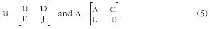
At this point, it seems to be more readable if we express our symbols B and A for a special case of Morishima–von Neumann model, using more familiar notation.¹¹ Employing the symbols in Krause (1980), we have

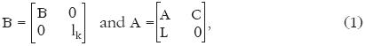
where B is the m by n material output coefficient matrix, l_k is the k by k identity matrix, A the m by n material input coefficient matrix, L the k by n labour input coefficient matrix, and C the m by k consumption basket matrix.¹² In Krause (1980), there is only one household process to reproduce each type of labour so that the number of household processes reduces from h to k. Note that in our framework, household activities to produce labour services are juxtaposed with the normal production processes in the matrices B and A. In our model, the zero elements of B and A for this special case can be positive, thus allowing for durable consumption goods, joint production of labour services, and direct labour inputs to produce labour services. Moreover, in our model, the number of columns of C need not be k, admitting of alternative household activities to produce labour services when k<h.

Now it is possible to select any commodity or a type of labour as the standard of value because goods and labour are treated in a completely symmetric way. Here, however, we choose a type of labour as the standard and let it be the i–th element among the (m+k) rows of B and A (m < i < + k). We give our definition of labour values as follows.

Definition of values for our general model: Values in a general input–output model are nonnegative magnitudes assigned to commodities (including normal commodities and various types of labour) such that the value of the standard labour be maximized under the condition that the total value of the output of each possible process should not exceed that of the input. When calculating the total value of the input of a process, unity is assigned to the direct input of the standard labour.¹³

Our productiveness assumption here is

Productiveness Assumption: There exists an such that:

 

where is the Euclidean space of dimension (n+h), and e_[i] is the (m+k)– column vector whose i–th entry is unity with all the remaining elements being zero.

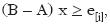
This assumption tells us that it is possible to organize an economy–wide production plan in which more than one unit of i–th labour service is produced as net output. Having defined values as above, we can now explain how to compute values in a systematic way. Let us first define the following vectors:

 

 

The vector Λ ^[i] is the vector of values with i–th element (labour) being the standard of value, and the entry stands for the value of commodity j with i–th labour as the standard of value. On the other hand, is Λ^[i] with its i–th entry replaced by unity so that it can embody the requirement that unity is assigned to the direct input of the standard labour. Our definition above is rewritten like this:

Find out Λ^[i] > 0 such that should be maximized

subject to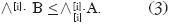

 

The constraint in this problem can be transformed first through adding to both sides, then multiplying both sides by nonzero nonnegative scalar v, yielding

 

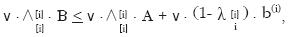
where b ⁽ⁱ⁾ is the i–th row of B. Then, we set

 

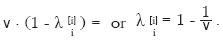
This normalization yields as our constraint

 

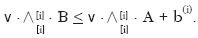
Since we have from our normalization, maximizing v is equivalent to maximizing . Writing simply as a variable vector q, thus q_i = v, we have the linear programming problem (LP):

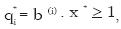
(LP) max q_i subject to q' . B < q' . A + b ⁽ⁱ⁾ and q' .

 

Finally, the values can be calculated as

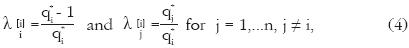
where q* is an optimal solution to (LP).
Dual to (LP) above is the problem (DP):

(DP) min b ⁽ⁱ⁾ . x subject to Bx > A x + e_[i] and x

Thanks to our Productiveness Assumption, the problem (DP) has an optimal solution, and its optimal value is not less than one by the very formulation of the problem. By use of duality in linear programming, it follows that

and we have shown in Fujimoto (2009) that in fact,

¹⁴

And this fact was used to discuss the existence of exploitation in Fujimoto (2009) in relation to prices and wage rates. The rate of exploitation for labour type i is given

as a positive magnitude when

. ¹⁵

 

4. REDUCTION TO A COMMON UNIT

There may be at least two reasons for the necessity of reduction of heterogeneous labour to a common unit. First, we wish to know the overall rate of exploitation for the whole working class without using the actual employment data. Second, we may have to construct a model with one homogeneous labour, given disaggregated data based upon heterogeneous labour.

Now we are ready to propose a method of reduction of heterogeneous labour to a common unit or abstract labour. To do so, we have to make more restrictive our model explained in the previous section. That is, our matrices B and A are represented as:

Here A is the m by n material input coefficient matrix, B the m by n material output coefficient matrix, C the m by h consumption basket matrix, D the m by h matrix of durable commodities remaining from C after one period, E the k by h matrix of direct labour inputs in household activities, F the k by n labour service output matrix from normal production processes, L the k by n labour service input matrix in the normal production processes, and J the k by h labour service output matrix from household activities. We assume that F = 0, and that the matrix J has a special form as follows:

 

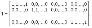
Thus, there is no joint production of labour services among all the household activities. It should be noted again we have made one more restrictive assumptions that labour services are produced only in household activities, i.e., F = 0.

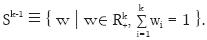
Our way of finding reduction ratios proceeds like this. First we select a row k–vector

, where S^k–1 is the simplex of dimension (k – 1), i.e.,

Using this α as a vector of conversion rates, we reduce our matrices B and A to

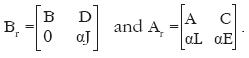
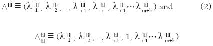
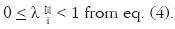
In this modification, various types of labour inputs in each process are "fused" into one scalar, and the size of two matrices B_r and A_r are now (m+1) by (n+h). With B_r and A_r given as data, we calculate labour values Λ ^[m+1], by solving (LP) and using eq.(4).¹⁶ Denote simply by Λ the m–vector formed by the first m elements of Λ ^[m+1]. This Λ represents the values of normal commodities in terms of fused labour. The inequality constraint (3) now turns into

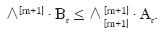
From this, we get

 

where at least one strict equality holds because we maximize subject to this constraint and F = 0.

Now the last element of the vector Λ ^[m+1] shows the value of fused labour with the fused labour being the standard, and we know as has been found in the previous section.

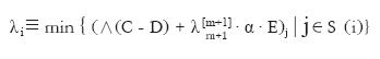
We are then able to calculate the value of each labour type in terms of fused labour. The row h–vector 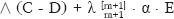means the vector of values in terms of fused labour actually consumed in household activities. Since the matrix J is of the supposed special form, the value of i–type of labour is obtained as the minimum of the elements of which correspond to the columns containing unity in the i–th row of J. More precisely, when we define the set S(i)

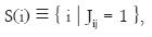
the value of i–type labour service in terms of fused labour, λ_i, is

We write w ≡(λ₁, λ₂,..., λ_k), and assume in addition that w ≠ 0.¹⁷ Normalize w ≠ 0 so that the sum of its elements is unity, i.e., the normalized vector .¹⁸ Since a solution to (LP) may not be unique, we have a correspondence from S^{k– 1} into itself. The image set f(α) is compact and convex, and the correspondence is evidently upper semi–continuous.

Therefore, Kakutani fixed point theorem guarantees the existence of a vector such that .

This implies that we can find conversion rates which are proportional to values in terms of fused labour. That is, pα = w, where p is a positive scalar. From (6) and one strict equality therein, we have . Then, the rate of exploitation of i–type of labour in terms of fused labour is given as:

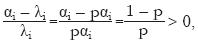
which is shown to be common among all types. With this property just stated, α*L may be called "abstract" labour, not fused labour in a naïve way.

As the reader may have noticed, we can rescale α* as we like. Thus, when we set a new α** ≡ cα* so that cα*_j = 1with a positive scalar c, it may be interpreted as choosing j–type of labour service as a common unit. Any type can be a common unit so long as α*_j > 0.

At this point, it is better to show that our reduction method includes that of Krause (1981) as a special case. In his model, B = I (the identity matrix) with m = n, D = 0, E = 0, and J = I (the identity matrix) with k = h, referring to our model (5) and his (1). Besides, the inequality (3) in the definition of values becomes an equality.¹⁹ Hence, our fixed point property becomes an eigenvalue problem

The standard reductions explicitly represented in Krause (1980) for models with joint production are also special cases of ours. To have α strictly positive, Krause (1981) assumes that two matrices M ≡ A + CL and H ≡ L(l – A)^–1C to be Sraffa matrices, which is weaker than irreducibility or indecomposability.²⁰ It seems natural, however, to allow α to be a nonnegative and nonzero vector, allowing for zero conversion rates for a set of labour typeS.

 

5. A NUMERICAL EXAMPLE

Let us use an example in Bowles and Gintis (1977) to show how our approach works. In their example, there are four normal commodities and three types of labour services: m=n=4 and k=h=3. The data therein given as Table 1 in Bowles and Gintis (1977) are

 

 

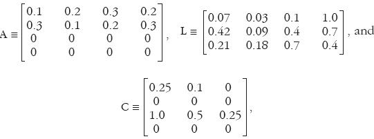
B = l₄, J = l₃, D = 0, E = 0, and F = 0, where the symbols are those in eq. (5). Bowles and Gintis²¹ named the four commodities "Food", "Steel", "Housing" and "Mercedes", and three types of labour services "Supervisory", "Primary" and "Secondary".

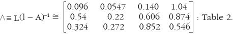
Their labour values of commodities (Table 2 in Bowles and Gintis)²² are

 

 

Their labour contents within each type of labour (Table 3 in Bowles and Gintis)²³ are

 

 

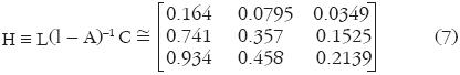
The Frobenius root of this matrix is µ(H) = 0.723 < 1. Therefore, as Potron (1913) and Krause (1981) proved, the equilibrium rate of profit is positive if the wage rate of each type of labour is exactly equal to the money value of its consumption basket.

To show that Bowles and Gintis (1977), Potron (1913), and Krause (1981) all made a wrong interpretation about the matrices Λ and H above, let us here compute the "correct" labour values in terms of "Secondary" labour based upon "conventional" method a la von Neumann. First we create the augmented input coefficient matrix A⁺ which includes in each process the necessary material inputs to employ "Supervisory" and "Primary" labour, i.e.,

 

 

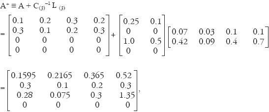
where C ₍₃₎ and L ₍₃₎ are the matrices C and L with the 3rd column and the 3rd row removed respectively. Then, the traditional way to calculate the labour values of normal commodities is by

 

 

where is the vector of values of normal commodities in terms of "Secondary" labour, L₃ the 3rd row of the matrix L. It is clear that the "correct" values are greater than those obtained by Bowles and Gintis (1977), the 3rd row of Table 2 above. This is simply because the requirements through the use of direct labour in each process are neglected.

Now let us proceed to our own way. Our matrix B is the 7 by 7 identity matrix I, while A becomes

 

 

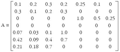
Our Productiveness Assumption in section 3 is satisfied by

where a prime stands for transposition of the vector.

In the special case here without joint production, the linear programming problem (LP) is solved by the following:

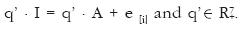
The solution q to this equation, with i=5 ("Supervisory" labour), i=6 ("Primary" labour), and i=7 ("Secondary" labour) respectively, are approximately

(0.348 0.184 0.502 1.964 1.589 0.286 0.126),
(1.662 0.796 2.221 50.24 2.637 2.277 0.555), and
(1.791 1.027 2.970 5.946 3.418 1.664 1.742).

Hence, by use of eq. (4), we compute the labour values in terms of labour type i=5,6 and 7, respectively, as:

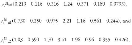
We can here see at once that the values of normal commodities in terms of "Secondary" labour, i.e., the first four elements of Λ^[7], coincide with those computed above in the conventional way, i.e., eq. (8). This is natural enough because of our definition eq. (3) with the strict equality holding and B being the identity matrix I. It can be seen that all the labour values of commodities turn out larger than those in Table 2 by Bowles and Gintis,²⁴ again because they neglected necessary labour via the inputs of other types of labour.²⁵ Incidentally, if we adopt the method in Fujimoto and Opocher (2010), to tell if a type of labour is more skilled than another, "Supervisory" labour is the most skilled and the "Secondary" labour the least.

When each type of labour receives their respective no–savings wage rate, we can calculate the rates of exploitation for individual types as

 

 

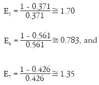
We have again strikingly different results from those by Bowles and Gintis,²⁶ in which the rate of exploitation for "Supervisory" labour is negative, i.e., –46%: that rate here is positive and 170%, the largest among three rates. This discrepancy comes from their arbitrary weights, actually equal weights, given to labour types when converting labour hours to some common unit. If we look at the values closely, the labour contents of housing (commodity 3) in terms of "Supervisory" labour is as low as 0.316, while those in terms of "Primary" labour and "Secondary" labour are 0.975 and 1.70, respectively: the latter are much greater. So, the value of "Supervisory" labour in terms of itself is small, though one unit of "Supervisory" labour consumes housing as large as 1.0 unit.

The reader is reminded that in order to calculate the rates of exploitation for individual types of labour, we need no data on how many workers of each type are employed, nor conversion of various types of labour to abstract labour (or a common unit).

And yet, we can actually construct our abstract labour following the method in Krause (1981) for the above special case. All we need is to find out the Frobenius root µ(H) and the row eigenvector associated with it for the matrix (7), i.e., H ≡ L(l – A)^–1 C. They are computed as

Hence, the uniform rate of exploitation is

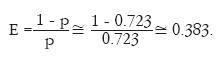
The common rate of exploitation is by far smaller than the individual rates of exploitation obtained above. This is because labour services of other types are regarded as normal commodities, horse/cow work, or even slaves' toil when we calculate the value of a particular type of labour in terms of that labour. In a sense, that type of labour is dictatorial in realizing the minimum amount of labour of the type while producing one unit of net labour service of the same type, i.e., in determining its value with the standard being its labour type. This is a weak as well as interesting point in our definition of values of individual heterogeneous labour types. On the other hand, when we reduce various types of labour services to abstract one, each type enters commodities as well as labour services on equal terms, i.e., no slaves at all, thus increasing the amount of necessary labour in terms of abstract labour, which implies a smaller rate of exploitation. Indeed, the notion of abstract labour should be useful to combine the whole spectrum of heterogeneous labour into one working class.

 

6. A STILL MORE GENERAL MODEL

A remaining problem is how we can treat more general models in which household activities can produce various labour services jointly, and household activities may require labour services as direct inputs. This we explain here in this section in a teleological manner. Let α be again a semi–positive row k–vector in the simplex of dimension (k–1), i.e., . Some more symbols are defined as follows:

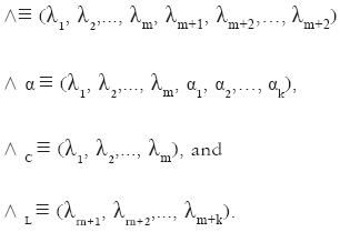
In this section, superscripts are left out from Λ's.

To obtain the reduction ratios in a general model, we first consider

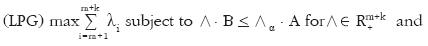
Λ L = p . α for some nonnegative scalar p.

Here α is a parameter vector to the problem (LPG). The meaning of the problem is that we should maximize the sum of values of all the labour services while the total value of outputs is not larger than that of inputs in each process / household activity with the direct labour inputs being given the weights represented by α. One more constraint tells us that values of labour services are proportional to the elements of a given parameter vector α. Substituting this requirement into the first constraint, the problem becomes

 

 

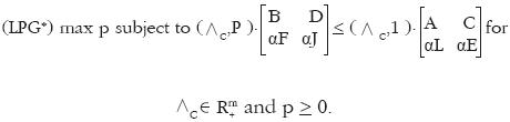
Note that here E and F are now not necessarily the zero matrix, and J is of a general type.

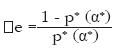
Exactly in the same way, this problem (LPG*) has a feasible vector by virtue of our Productiveness Assumption, and an optimal solution p* (α) is less than one. This p* (α) can be positive under a certain condition.²⁷ Finally, the desired reduction ratios α* are to be obtained by solving

max p* (α) for .

And the uniform rate of exploitation is defined by

 

 

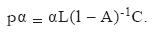
Our method in this section may include the reduction ratios hitherto proposed as special cases. Let us take up the case where B and A are m by m square matrices, and the nonnegative inverse (B – A)^–1 exists; D, E, and F are all zero matrices; h=k, and J= l_k. In this case, it follows from the two constraints of (LPG*) that

 

 

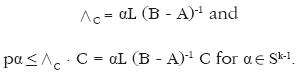
From Perron–Frobenius theorem, we know that the maximum p is realized when it is the Perron–Frobenius root of L(B – A)^–1 with α being its associate eigenvector.

 

7. REMARKS

An alternative linear programming problem to (LP) above can be obtained directly from (3):

where A_[i] is A with its i–th row replaced by zero vector, and a ⁽ⁱ⁾ is the i–th row of A. And the dual one is:

Using these, we are able to obtain the same propositions. This problem (LP2) gives a more direct interpretation of labour value, and can be an alternative definition. We have, however, adopted a traditional definition of direct and indirect requirement.

In sum, we have shown a method to discover the reduction ratios which Marx described in Capital I, for a general model with joint production in production processes as well as household activities, and durable consumption goods. A mathematical key is the generalized eigenvalue problem. Supposing such reduction ratios, Marx was able to conceive the one working class as a whole in spite of the heterogeneity of labour power, and an equal rate of exploitation among all the types of labour services is observed. It is now easy to tell which labour type is more "skilled" than another.

In a sense, the method explained in section 3 is a "separatist" method, while the reduction to abstract labour presented in section 4 is a "unionist" approach. Surely the latter is more favorable to Marx because all the workers are regarded as "friends" in a capitalist production system. The separatist method does not necessarily think of workers of different types as "enemies" to each other, but certainly not as "friends".

One final remark is concerned with the fact that labour values can be computed by using abstract labour, while prices are described by using heterogeneous labour services.

Our method is applicable to a theory of aggregation of commodities into composite ones without depending prices in a model with joint production. This is another theme we will tackle with in the future research.²⁸

 

NOTAS

* Acknowledgments: thanks are due to professor Dr. Alejandro Valle Baeza who had introduced this journal to the authors, and to our friend professor Dr Ulrich Krause for his encouragement. The authors are grateful to the referees who have provided useful comments and suggestions to improve this article.

¹ K. Marx, "Wages, Price and Profit", speech in 1865, published in 1898: Section 7; K. Marx, Capital I, the original German edition in 1867 [www.marxists.org/archive/marx/works/1865]         [ Links ].

² K. Marx, Capital I, 1867, op. cit., Part 1, Chapter 1, Section 2, p. 12.

³ M. Potron, "Quelques propriétés des substitutions linéaires à coefficients > 0 et leur application aux problèmes de la production et des salaires", Annales Scientifiques de l'É.N.S., 3e série, t. 30, 1913, pp. 53–76.         [ Links ] See also K. Mori, "Maurice Potron's linear economic model: A de facto proof of 'fundamental Marxian theorem'", Metroeconomica, vol. 59, 2008, pp. 511–529.         [ Links ]

⁴ S. Bowles and H. Gintis, "The Marxian theory of value and heterogeneous labour: a critique and reformulation", Cambridge Journal of Economics, vol. 1, 1977, pp. 173–192.         [ Links ]

⁵ I. Steedman, "Heterogeneous labour and «classical» theory", Metroeconomica, vol. 32, 1980, pp. 39–50.         [ Links ] U. Krause, "Abstract labour in general joint systems", Metroeconomica, vol. 32, 1980, pp. 115–135.         [ Links ]

⁶ U. Krause, "Heterogeneous labour and the fundamental Marxian theorem", Review of Economic Studies, vol. 48, 1981, pp. 173–178.         [ Links ]

⁷ See K. Mori, "Maurice Potron's linear economic model...", op. cit., p. 523. It seems to the authors, however, that Potron (1913) had no notion of exploitation.

⁸ T. Fujimoto and A. Opocher, "Commodity content in a general input–output model", Metroeconomica, vol. 61, 2010, pp. 442–453.         [ Links ] Y. Fujita, "On the reduction problem in Marxian value theory", Fukuoka University Review of Economics, vol. 30, 1985, pp. 43–49.         [ Links ]

⁹ T. Fujimoto, "The concept of exploitation in a general linear model with heterogeneous labour", Investigación Económica, vol. 68, UNAM, 2009, pp. 51–82. Some notational typos remain.         [ Links ]

¹⁰ M. Morishima, Equilibrium, Stability, and Growth: A Multi–sectoral Analysis, Oxford University Press, 1964.         [ Links ] See also M. Morishima, Marx's Economics: A Dual Theory of Value and Growth, Cambridge University Press, 1973.         [ Links ]

¹¹ The readers who are accustomed to Leontief models are referred to T. Fujimoto, "The concept of exploitation in a general linear model with heterogeneous labour", op. cit., for an explanation, easier to grasp, of our model.

¹² U. Krause, "Abstract labour in general joint systems", op. cit., used the symbol F in place of our C.

¹³ Among a plural number of solutions, we adopt those which realize the maximum number of equalities in the constraints. And yet, a solution may not be unique.

¹⁴ Proposition 2 in T. Fujimoto, "The concept of exploitation in a general linear model with heterogeneous labour", op. cit., p. 63.

¹⁵ When = 0, the rate of exploitation can be regarded as infinitely large if a worker of this type is employed at a positive wage rate.

¹⁶ For Λ ^[m+1], see eq. (2) above. The index [i] is here replaced by [m+1].

¹⁷ It is sufficient to assume that there exists at least one type of labour service, simple or unskilled, which is required directly or indirectly to produce each type of labour service.

¹⁸ Since this vector depends on the parameter a chosen at the start, it is written as in the text.

¹⁹ This is related to the non–substitution theorems. See T. Fujimoto et al., "A complete characterization of economies with the non–substitution property", Economic Issues, vol. 8, 2003, pp. 63–70 [www.economicissues.org/archive/volindex.html]         [ Links ].

²⁰ In the case of joint production, U. Krause, "Abstract labour in general joint systems", op. cit., assumes the system (A, B, L) is connected. For indecomposability, see T. Fujimoto and F. Ekuni, "Indecomposability and primitivity of nonnegative matrices", Política y Cultura, núm. 21, 2004, pp. 163–176.         [ Links ]

²¹ S. Bowles and H. Gintis, "The Marxian theory of value and heterogeneous labour: a critique and reformulation", op. cit., p. 182.

²² Ibid., p. 183.

²³ Ibid., p. 184.

²⁴ Ibid., p. 183.

²⁵ Based upon the matrix S. Bowles and H. Gintis, "The Marxian theory of value and heterogeneous labour: a critique and reformulation", op. cit., gave two definitions of exploitation rate for each labour type. Both are, however, either inadequate or arbitrary as are criticized by Catephores. In short, they had to make up for the underestimation of values. See G. Catephores, "On heterogeneous labour and the labour theory of value", Cambridge Journal of Economics, vol. 5, 1981, pp. 273–280.         [ Links ]

²⁶ S. Bowles and H. Gintis, "The Marxian theory of value and heterogeneous labour: a critique and reformulation", op. cit., 184.

²⁷ See footnote 18.

²⁸ M. Morishima and F. Seton, "Aggregation in Leontief matrices and the labour theory of value", Econometrica, vol. 29, 1961, pp. 203–220.         [ Links ]