


 nueva página del texto (beta)
 Inglés (pdf)
 Artículo en XML
 Referencias del artículo
 Enviar artículo por email
 Citado por SciELO
  Similares en
SciELO
Similares en
SciELO 
 Permalink
Introduction
The FEFF spectroscopy package was originally made to calculate x-ray absorption fine structure (XAFS) (Rehr et al., 2009) by using a real space Green function (RSGF) formalism, which involves obtaining an electron’s Green function in a condensed matter system (Rehr & Albers, 1990). The name of the package is a reference to the effective curved-wave scattering amplitude (f eff ), which plays an important role in the description of electron interactions with the atoms that constitute a material (Mustre de León, 1991). The Green can be expressed as a series that involves real space multiple scattering (RSMS) segments over the different atoms in the system, which produces an approach that is computationally fast and numerically accurate. Other important response functions that describe the interaction of electromagnetic waves and condensed matter systems can be obtained through the same type of expansion, which has been used to add other types of spectroscopic quantities of interest to the software’s capabilities (Rehr et al., 2010).
For this work, FEFF 9 is used to first calculate copper’s photo-absorption cross section (or the imaginary part of the FSA for each electronic shell), from which we obtain an estimate of the imaginary part of the dielectric function as a function on incident photon energy, which then leads to the rest of the optical constants by means of the relations described below.
Purpose of this work
The main purpose of this work is to partially update the results of the author’s contribution to a previous work (Prange et al., 2009), which originally were done using the FEFF package version 8, specifically the optical constants of metallic copper.
A secondary purpose, which is similar to the work by Prange et al. (2009), is a proof of principle test of the adequacy and limitations of the theory behind FEFF version 9 to calculate values of the optical constants and photoabsorption spectrum for the far ultraviolet to the lower energy region of the x-ray spectrum, i.e., above 10 eV and below 1000 eV approximately (the soft x-ray region).
Basic theory
Electromagnetic radiation can be described by quantum mechanics in terms of light particles or photons, each of which carries an energy dependent on its frequency ν or wavelength in vacuum λ, which is given by Planck’s relation:
where h is Planck’s constant, ħ = h/2π is the reduced Planck constant, c is the speed of light in vacuum, and k = 2π/λ is its wavenumber (Sakurai, 1967).
When electromagnetic radiation interacts with ordinary condensed matter, there is a quantum mechanical probability for it to be absorbed by an atom or an ion, followed by the emission of a photoelectron. This is characterized by an effective area, or photo-absorption cross section σ(E), that an atom presents to an incident photon. The cross section σ(E) is a function of the energy E of the photon, and it can be obtained by evaluating Fermi’s Golden Rule (Sakurai, 1967):
where m is the mass of the electron; r
e
=e
2
/mc
2
is the classical electron radius, with e the electric charge of the electron; I (F) denotes the initial (final) state of the system of the atom or ion, photon, photoelectron, and surrounding atomic environment before (after) the absorption of the photon; E
I
(E
F
) indicates the energy of the corresponding state; and
In terms of the electron Green function operator G(E), the cross section can be expressed as:
In this expression, all the information concerning the final states is within the Green function (Rehr & Albers, 1990). The Green function describes the propagation of the photoelectron within the condensed system; and in real space, it can be expanded into a series representing the initial absorption plus subsequent scatterings from the atomic environment. FEFF calculates photo-absorption cross sections of molecules and clusters of atoms for x-ray photons (Rehr et al., 2009) by means of this RSGF formalism. The contribution from the multiple scatterings in the atomic environment constitutes the x-ray absorption fine structure (XAFS) (Rehr & Albers, 2000).
The XAFS can be separated into two regimes due to differences in the physics involved:
1.The x-ray near-edge absorption fine structure (XANES), which refers to the fine structure approximately up to 50 eV-60 eV from the onset of the absorption of the photon (the absorption edge); in this region, an accurate calculation requires a high order of the RSMS expansion, which is done by full multiple scattering (FMS) in which the RSMS expansion is formally carried to infinite order on a large cluster of atoms (Ankudinov et al., 1998).
2. The region (above the XANES) of the extended x-ray absorption fine structure (EXAFS), which covers a few thousand eV (2500 eV-3500 eV) above the edge, after which the fine structure disappears; this is accurately calculated by the RSMS approach to finite order (Rehr & Albers, 2000).
When analyzing the process of elastic photon scattering by atoms, a similar equation is obtained for the relative amplitude f(E) of the scattered electromagnetic wave with no deviation of the scattered photon (i.e., with q = 0), the forward scattering amplitude (FSA). The FSA is a complex-valued function, and it can be written as
with f T as the Thomson scattering amplitude, which is approximately equal to the atomic number Z of the element, and the rest is the anomalous scattering amplitude (Sakurai, 1967).
If the initial state is the ground state, then f’’(E) is given by:
which relates it to the photo-absorption cross section:
this implies that the FSA possesses fine structure the same way σ(E) does, and thus it can be calculated in the same fashion as the absorption cross section (Ankudinov & Rehr, 2000).
The FSA is also related to the dielectric response of a substance by means of the complex dielectric atomic polarizability (Jackson, 1975; Vedrinskii et al., 1992):
and the dielectric susceptibility χ e :
with N as the number density of atoms. The susceptibility is then related to the complex dielectric constant, ε(E):
This equation connects the photo-absorption cross-section to the imaginary part of the dielectric function ε 2 :
The real part of the dielectric constant ε 1 can be obtained then via a Kramers-Kronig relation (KKR) (Jackson, 1975):
where P indicates the principal part of the integral.
Other functions, or optical constants, can then be derived from the dielectric constant (Jackson, 1975). The energy loss function is the negative of the imaginary part of the inverse dielectric constant:
The complex index of refraction n ref for non-magnetic substances is the principal branch of the complex square root of the dielectric constant:
from which the normal incidence reflectivity R, or reflectance, is calculated by:
and from κ(E) the absorption coefficient µ(E) is obtained:
The absorption coefficient µ(E) describes the attenuation of the intensity of a beam of electromagnetic radiation when it crosses a material medium; that is, if a beam initial intensity I 0 travels a distance x through a medium, the resulting intensity I is (Jackson, 1975):
These will be the main dielectric constants which will be the focus of this article. Over the next section, a summary of some of the more subtle aspects of the theory will be covered.
Other theoretical considerations
Several theoretical considerations are needed to describe electronic interactions in materials. Some are important to describe the methodology of this work; therefore, a summary of a few of them is provided here, leaving the details to the references.
Electron configuration and scattering potentials. To calculate equations 2, 3, or 5, the initial and final states I and F are needed. These require a calculation of the electron configuration of the atoms inside a material. When a photon is absorbed by an atom, its final states F contain a vacancy when a photoelectron is ejected. This photoelectron scatters from the atoms in the material by interacting with the potential produced by their electron configurations. These configurations are calculated by FEFF, by initially solving the Dirac equation numerically for free atoms (Ankudinov et al., 1996).
The free atomic charge distributions are then put into coordinates describing the locations of atoms in a cluster, and any overlap of charge distribution is then used to recalculate new potentials, giving new electron distributions for each type of atom. This procedure is iterated in a self-consistent field (SCF) manner until convergence is achieved (Rehr & Albers, 2000). FEFF requires only the radius of the cluster to be able to perform all these computations automatically.
Core-hole and screening. The initial and final electron configuration of the absorbing atom differ in general, as a core-hole is left after the ejection of the photoelectron. The photoelectron interacts with this vacancy. There are several prescriptions on how to treat the core-hole (Rehr & Albers, 2000). FEFF 8 allowed two options: no core-hole and the final state rule, for which the electron configuration is calculated with a vacancy in the electronic subshell from where the photoelectron originated (Rehr & Albers, 1990). FEFF 9 added a third option: a random phase approximation (RPA) screened hole, in which the electrostatic screening of the hole by the other electrons is partially accounted for. The treatment chosen is given as a parameter value to FEFF (Rehr et al., 2010).
Multi-pole self-energy. The photoelectron itself behaves like elementary excitation of the material; it is considered a quasi-particle, with a self-energy that describes its propagation in the interstitial region between atoms or ions of the material (Rehr & Albers, 2000). The self-energy is a complex function, and an accurate treatment requires it to be modeled with several poles in the complex energy plane. This is a more accurate model for treating the photoelectron and the XAFS produced since it scatters by the atoms inside the material. This option must be turned on to be included in the calculation by FEFF 9 (Kas et al., 2007), and it is absent in FEFF 8.
Spectral convolution and many body effects. The absorbing atom and photoelectron are a system made of several particles and should be considered as a whole: they are a many-body system. After a photon is absorbed, and the photoelectron is ejected, the ion that is left may be in an excited state. The energy of the photon is conserved in the process and must be divided between the photoelectron and the remaining ion. Thus, the photoabsorption may result in a photoelectron with many possible energies than a direct transition in which the ion is left with its lowest possible energy. The full contribution to the absorption can be obtained from a spectral convolution of values of cross sections for different photoelectron energies (Campbell et al., 2002; Rehr & Albers, 2000). Options to include these effects in a calculation are available in FEFF 9, but not in FEFF 8 (Rehr et al., 2010).
Temperature effects. At finite temperature, the positions of the atoms in a condensed matter system are not fixed because of thermal motion (Ashcroft & Mermin, 1976). This attenuates the fine structure contribution from long scattering paths (Rehr & Albers, 2000). This can be approximated by a Debye-like model for thermal motion as a first approximation (Rehr & Albers, 1990), which requires as input the Debye temperature of the material and a temperature to assume in the calculation.
Materials and Methods
Since this is a theoretical and computational approach to obtaining an estimate of the optical constants, the only material object needed was an adequate computer to allow for a speedy calculation. For that, an MSI GT72 2QE notebook computer was used, with an Intel 4720HQ CPU, 16 GB of 1600 MHz DDR3 core RAM, and an NVIDIA GTX 980m 8GB VRAM GPU; running 64 bit Windows 10, under the MSYS2 64 bit environment, which is a 64 bit Linux-like subsystem running MS-DOS commands with a Linux type behavior and command syntax. The FEFF code was version 9.6 with modifications by the author to allow for a larger than default range of the photon energy grid (see below for details), which is allowed by the license of the software. The code was compiled under MSYS2, using GNU-Fortran version 7.1.0 and Microsoft MPI version 10 to allow for the use of the multiple cores of the CPU for parts of the code that can run in parallel to speed up the calculations.
Copper was used as test material for the calculations because for x-rays it has large XAFS (Rehr & Albers, 1990, 2000), and because the complex structure of its optical constants in the energy region of 10 eV-120 eV make it a good test case for a theoretical prediction of these constants. The availability of values derived from the experiment of some of these constants obtained by Hagemann et al. (1975) also played a role.
The calculations were done for each electron shell and absorption edge of copper, except for the 4s valence electron (the N1 edge), since an atomic-like orbital did not converge for an atom embedded in a solid, and for which the band structure of copper is expected to play a large role. Instead for the 4s shell, a Drude approximation was used for its contribution to the dielectric constant to provide a background at low photon energies (Ashcroft & Mermin, 1976):
The value for Γ was obtained from parameters for copper given by Ashcroft & Mermin (1976).
For each of the other electronic shells and absorption edges, the FEFF code was used to calculate: a) photo-absorption cross sections in the near-edge region (x-ray near edge structure, or XANES) for which, due to strong scattering up to about 50 eV, a FMS calculation is necessary b) photo absorption cross sections for the extended x-ray absorption fine structure (EXAFS) region, above 50 eV up to around 3000 eV from the absorption edge, and for which a finite order RSMS converges rapidly and is therefore sufficient; and c) for the far region where no fine structure is observed and can be up to tens of thousands of eV above the edge, the imaginary part of the FSA with no fine structure is computed.
The energy grid for XANES was modified in the code to allow a calculation starting at an energy well below the edge and obtain a full graph of the onset of the absorption edge, or pre-edge region. The values of energy of the calculated XANES for every edge corresponded to a photoelectron wavefunction wave number of k = 10 Å-1 (ten inverse angstroms) below the edge and up to k = 5 Å-1 above the edge. FEFF by default calculates EXAFS from photoelectron wave number k = 0 Å-1, up to k = 20 Å-1; the energy grid was also modified to allow for calculation up to k = 30 Å-1 to ensure that all the fine structure would be present in a single graph. The calculation of the FSA was performed at an initial energy of 200 eV below the last value calculated for EXAFS, and it was performed with a spacing of 100 eV for one hundred points and a second calculation with a spacing of 1000 eV for another one hundred.
As there was some overlap between the values obtained by XANES using FMS and EXAFS using RSMS, and between EXAFS and the values from the FSA which did not include fine structure, it is required to provide a smooth transition from one calculation regime to the next, so that an interpolation between the two was done. That is, when two functions (F 1 (E), F 2 (E)) for a quantity F(E) corresponding to two modes of calculation overlapped, a value was obtained by means of a weight function w(E) such that w(E 1 )=1 and w(E 2 )=0, so that in the interval (E 1 , E 2 ) we take:
For a smooth function with zero derivatives at the end points (E 1 , E 2 ), the weight function was taken as:
this choice for w(E) is somewhat arbitrary, and it was chosen by the author because it makes the first derivatives at the end points continuous, i.e., the transition is smooth, without breaks in the slope of the graphs at the end points (E 1 , E 2 ). Other choices for w(E) are possible, and it is desirable that they preserve continuity of at least the first derivative at the same endpoints, but for the present work this choice was sufficient, since the function is used to switch from F 1 to F 2 in regions where the two functions are almost identical (see below). Other choices may be left for future analysis. For XANES and EXAFS, the values of E 1 and E 2 were chosen to correspond to a range of photoelectron wavenumbers from 3.5 Å-1 to 4.5 Å-1; these values correspond approximately to the transition from XANES to EXAFS, 47 eV to 77 eV respectively, above the edge (Rehr & Albers, 2000), and it corresponds to a region where the two visually resemble each other the most. The overlap between EXAFS and the FSA far from the edge was chosen as 200 eV solely to provide an overlap, since slight numerical differences in the algorithm for the two regions allowed for a small mismatch of the calculated absorption cross sections, which created a need for a smooth transition between the two.
For all the above calculations, a cluster of 135 atoms centered on the absorber was used for a SCF calculation of the atomic charge distribution and potentials; a cluster of 201 atoms was used to obtain the fine structure for XANES and EXAFS.
RPA screening was used for the core-hole, and a many-pole photoelectron self-energy was included (Kas et al., 2007). As discussed in Kas et al. (2007), this self-energy requires an estimate of the energy-loss function as input, with FEFF providing a very crude estimate by default; therefore, in order to provide for a better estimate, the calculations for the optical constants were done twice: the first run was done to obtain an estimate of the energy loss function to use for the second run. A spectral convolution was also done for EXAFS and XANES to account for many-body excited atomic state effects (Kas et al., 2007).
Finally, to account for temperature effects, 290 K was assumed, and a Debye temperature of 315 K was taken from Ashcroft & Mermin (1976).
The results for each edge were combined to obtain the imaginary part of the dielectric constant ε 2 (E), by interpolating from the FEFF calculation onto a user-defined photon energy grid with a logarithmic spacing between 0.001 eV and up to 100 eV, and a regular spaced grid with a step of 0.2 eV from 100 eV up to 50000 eV. A linear piece-wise interpolation was used for the values obtained for XANES and EXAFS. For the energy points derived from the FSA, a power law was fitted between each pair of consecutive points, which is equivalent to a linear fit of the logarithm of calculated values versus the logarithm of the energy: it is common practice to tabulate the logarithms of cross sections and values of the FSA far from an absorption edge as polynomial splines of the photon energy, e.g., as in the work by Elam et al. (2002). Thus, a linear interpolation of the logarithm of ε 2 (E) versus the logarithm of the energy was deemed sufficient since the values derived from FEFF were at most 1000 eV apart.
The real part of the dielectric function was then obtained at the midpoints of the user-defined grid by means of numerically evaluating the KKR integral (equation 11 of this article) as discussed in Jackson (1975). Special care had to be taken to ensure numerical convergence: trapezoidal numerical integration of the whole integrand (Press et al., 1992) was found to work well when the grid intervals were far from the value E, but when the values in the integrand are evaluated at less than a few tens of eV far from E, or if E is in the middle of the interval over which the integration is calculated, the trapezoidal rule was found to give inaccurate results; however, an exact integration formula can be explicitly obtained and evaluated assuming a linear piece-wise approximation for the numerator in the integrand. That is, if one has a function f(x) = mx + b, then:
This relation is correct even when x 0 is in the middle of the interval (x k , x k+1 ), and for the selected energy mesh was found to be sufficiently accurate, though computationally more costly; hence, it was limited to intervals within 25 eV of E.
The above procedure was implemented in a Fortran 90 computer program that read the corresponding files obtained from FEFF and carried out the interpolation of values onto the user defined grid to obtain a total contribution from every electronic shell to the imaginary part of the dielectric constant. This was written onto a file which was then used by another program to obtain the real part of the dielectric constant by calculating the KKR at the mid-points of every energy interval of the user defined grid, which would then combine it with the imaginary values of the dielectric constant to obtain the rest of the optical constants.
Results
The results of the above calculations are shown in the next figures, with comparison to values well known from the literature. For copper, the calculations are compared to data from Hagemann et al. (1975) for most of the optical constants. Values of the FSA for comparison are taken from Henke et al. (1993). In the key of the figures, Present work refers to the values derived from FEFF, HGK refers to data from Hagemann et al. (1975), and Henke corresponds to data from Henke et al. (1993).
In all figures, the values calculated from FEFF data and the values from the literature agree well for energies greater than approximately 100 eV, corresponding to the onset of soft x-rays. The theory behind FEFF (FEFF reference) is a theory for x-ray spectroscopies, and agreement for x-rays is expected. For values of the energy between approximately 10 eV and 100 eV, the agreement becomes more qualitative: peaks of local maxima, minima, and points of inflection appear at about the same values of photon energy, but the exact values of the quantities do not necessarily agree.
In Figure 1, the imaginary part of the dielectric function ε 2 (E) is shown. The values calculated in the present work are compared to data by Hagemann et al. (1975). It is seen that for values below 100 eV there are discrepancies, and values below 10 eV are large. In the region between 10 eV and 100 eV there is qualitative agreement in the general features. This is the region of transition between hard ultra-violet light (UV) to soft x-rays. Above 100 eV the two curves show much closer agreement.
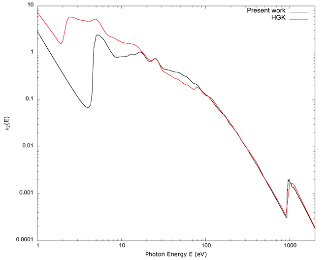
Source: Author’s own elaboration.
Figure 1 The imaginary part of the dielectric constant ε 2 vs. photon energy E. The line indicated as Present work is the calculated values derived from FEFF; the line indicated by HGK is from Hagemann et al. (1975). Notice the large difference between the calculated values from FEFF and those from Hagemann et al. (1975) below 10 eV, the qualitative agreement for energies in the range 10 eV-100 eV, and the quantitative agreement above 100 eV, corresponding to the onset of soft x-rays.
In Figure 2, the real part of the dielectric function ε 1 (E) obtained by the KKR from the imaginary part ε 2 (E) is shown. Note that the scales on the left and on the right of the graph are different. The one on the right is magnified to highlight small departures from a value of 1. Some of the same observations for the imaginary part apply here as well: below 100 eV, the agreement between the calculated values from FEFF and the data from Hagemann et al. (1975) are more qualitative, i.e., features like local maxima and points of inflection agree. Above approximately 100 eV the two graphs converge to a value of 1.
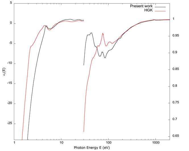
Note the use of different scales for the left and right portions of the graph. For each side, the two curves cover the same energy range.
Source: Authors’ own elaboration.
Figure 2 The real part of the dielectric constant ε 1 vs. photon energy E. As in Figure 1, the line indicated as Present work is from the values derived from FEFF; the line indicated by HGK is from Hagemann et al. (1975).
The negative of the reciprocal of the imaginary constant, -Im(1/ε), is shown in Figure 3. The values calculated from FEFF are compared to the values from Hagemann et al. (1975). In this figure, the two curves show the maxima and points of inflection of the two at the same values of photon energy between 10 eV and 100 eV, though the precise values of the curves can differ significantly. The agreement improves when photon energies correspond to x-rays, above 100 eV approximately.
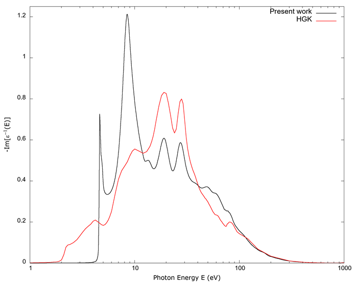
Source: Authors’ own elaboration.
Figure 3 The negative of the inverse of the dielectric constant ε vs. photon energy E. As in Figures 1 and 2, the line indicated as Present work is from the values derived from FEFF; the line indicated by HGK is from Hagemann et al. (1975). The values below approximately 10 eV do not agree, while between 10 eV-100 eV the agreement becomes qualitative. For energies above 100 eV, which corresponds to the onset of soft x-rays, the agreement improves.
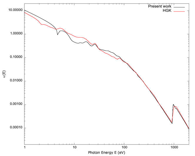
Figures 4 and 5 respectively show the real n and imaginary κ parts of the complex index of refraction. (Note the different scales for the left and right vertical axes in Figure 4.) As the case for Figure 2, the right axis is magnified to show small deviations from a value of 1. Figure 5 is plotted in a log-log scale to show a full spectrum like in Figure 1. The same qualitative agreement between the values from Hagemann et al. (1975) and the ones derived from FEFF are present in both.
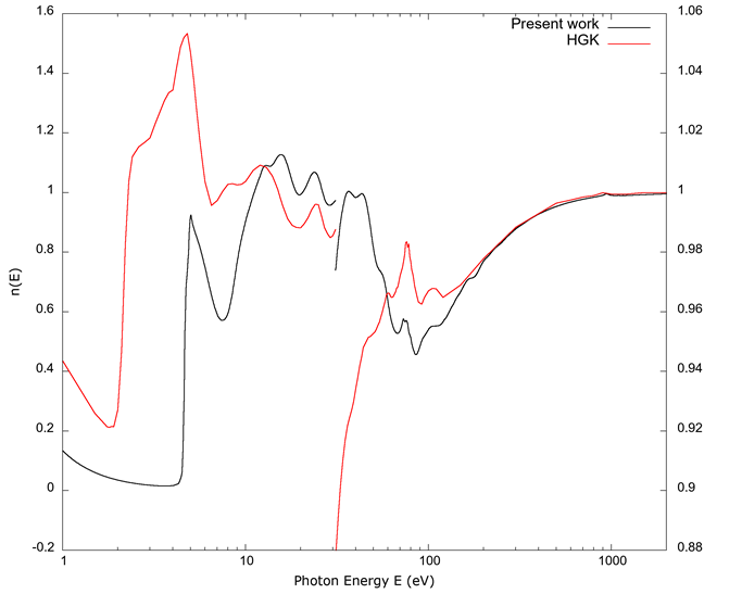
Source: Author’s own elaboration.
Figure 4 The real part n(E) of the complex index of refraction vs. photon energy E. As in Figure 2, the right side of the graph is magnified relative to the left to highlight small deviations from a value of 1. We can appreciate similar characteristics to those seen in Figure 2: the FEFF derived curve below approximately 8 eV does not agree with the values from Hagemann et al. (1975), while between 8 eV-100 eV the agreement is better, but qualitative. For energies above 100 eV, the two curves coincide within the resolution of the graph.
Source: Authors’ own elaboration.
Figure 5 The imaginary part κ(E) of the complex index of refraction vs. photon energy E. To be able to show a full spectrum, as in Figure 1, a log-log scale has been used. Values calculated from FEFF and those from Hagemann et al. (1975) offer a better general agreement than those of Figure 1 below 100 eV, and the agreement improves for energies above 100 eV.
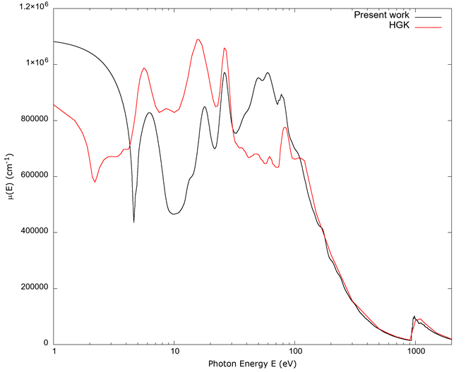
Figure 6 contains a graph of the absorption coefficient µ(E). The same general observations apply as in the previous figures: we have qualitative agreement for values below approximately 100 eV, and the agreement improves for energies corresponding to x-rays.
Source: Author’s own elaboration.
Figure 6 The absorption coefficient µ(E) vs. photon energy E. Values calculated from FEFF and those from Hagemann et al. (1975) qualitatively agree below 100 eV, and the agreement improves for energies above 100 eV.
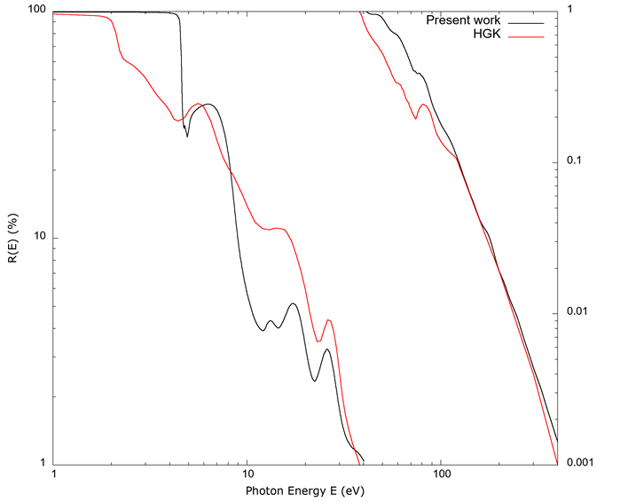
Figure 7 is a graph of the reflectance R (in percent %) as a function of photon energy. The reflectance is too high for FEFF derived values below 5 eV, and qualitative agreement with the data from Hagemann et al. (1975) is seen between that and 100 eV, with a closer match of the two curves above that value; the graph goes only to 400 eV, as Hagemann et al. (1975) reports values above that energy as equal to 0.
Source: Author’s own elaboration.
Figure 7 The normal incidence reflectivity R (%) as a function of photon energy E. This is on a log-log scale, with different ranges for the left and right portions of the curves. Data from Hagemann et al. (1975) were reported as a value of 0.000 above 400 eV, and thus the calculated values are not shown above that range of energy. The calculated reflectance is too high below 5 eV and only qualitatively agrees with the data from Hagemann et al. (1975) in the range 5 eV-100 eV, as in the previous graphs.
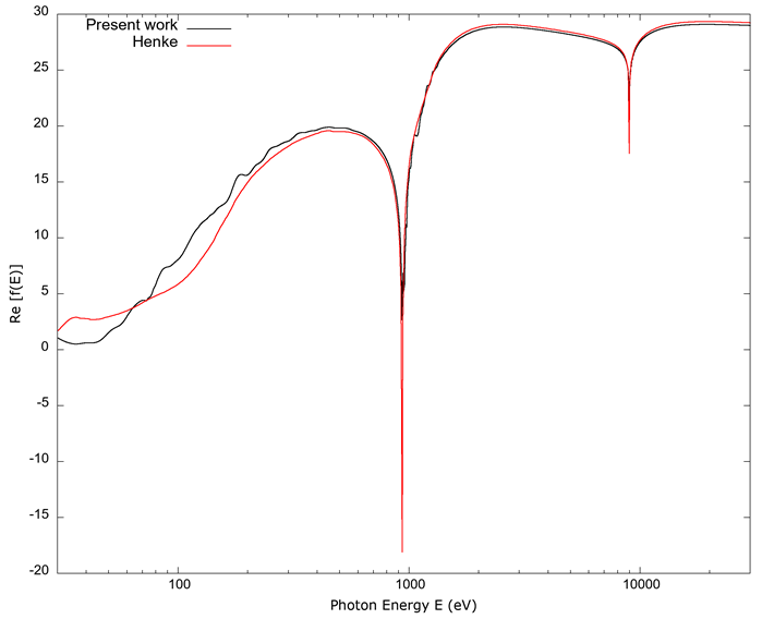
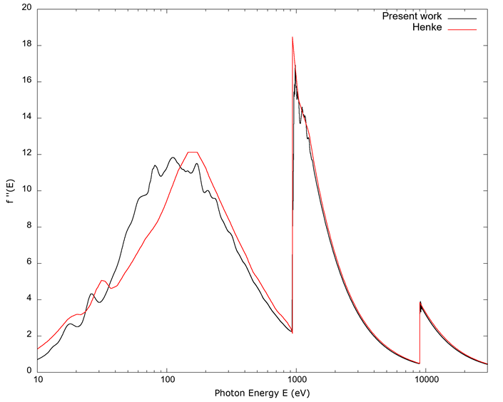
In Figures 8 and 9, the plots show, respectively, the real and imaginary values of the FSA obtained in the present work together with those from Henke et al. (1993); these values do not include fine structure, so complete agreement is not expected.
Source: Author’s own elaboration.
Figure 8 The real part of the FSA f’(E) vs. photon energy E. Values for Re[f(E)] from Henke et al. (1993) are only available above 30 eV, so the plot begins at that value. Both curves agree within a small fraction of each other for hard x-rays. For the region in the transition from the hard UV to soft x-rays, 30 eV-300 eV, there is a more pronounced difference; however, the data from Henke et al. (1993) does not include fine structure and has larger uncertainties in that region, and FEFF does not calculate band structure, so the disagreement is not unexpected.
Source: Author’s own elaboration.
Figure 9 The imaginary part of the FSA f’’(E) vs. photon energy E. The data from Henke et al. (1993) begins at 10 eV. Both curves agree above 1000 eV, but as observed in the caption to Figure 8, the uncertainties in the data from Henke et al. (1993) are larger for soft x-rays and the UV than for x-rays and do not include fine structure, while FEFF does not calculate band structure, so partial disagreement is not unexpected here.
Discussion
As can be seen in the figures, the optical constants of copper as calculated from FEFF 9 are accurate in the x-ray regime, for which the theory behind the software is well suited. However, for photon energies corresponding to the UV, there is qualitative agreement between approximately 10 eV and up to about 100 eV, and the agreement is only suggestive below that energy interval. This is still in conformity to the results from Prange et al. (2009), which involved version 8 of FEFF, with some differences in the exact values computed there. The accuracy and numerical precision of the software has not changed in FEFF 9, so these differences are the result of the additional physics involved in the computation. An exact comparison was not made in this work, but it is contemplated for the future, including other elements for which values are tabulated in the work by Hagemann et al. (1975).
These results are not unexpected. FEFF was designed for x-ray spectroscopies, for which more tightly bound electrons contribute, and thus the theory does not address the band structure of valence electrons in a solid. However, the qualitative agreement (coinciding maxima and minima, and points of inflection) in the region of approximately 10 eV-100 eV suggests that the density of states (DOS) in the energy region close to the valence and conduction bands is close to the correct values, and both FEFF 8 and FEFF 9 are designed to calculate these accurately (Ankudinov et al., 1998; Rehr et al., 2010). This suggests that it may be possible to modify the package to obtain more accurate information.
For copper, the band structure from the 4s electron is the main contributor below 10 eV. Results from FEFF failed to converge properly for this electronic shell, so the contribution from this electron was calculated in a crude manner by means of the Drude term of equation 16, mostly to provide a background for the rest of the electron orbitals; given the crudeness of the model, only broad agreement was expected for this electronic shell. The Drude term for the 4s electron explains the high reflectivity seen in Figure 7, as that model gives a plasma frequency for copper corresponding to approximately 7.4 eV. A Drude-type metal should be transparent for photons above approximately that energy (Ashcroft & Mermin, 1976), and we see the calculated reflectance dip in value as the energy approaches 7.4 eV. A more accurate treatment for the 4s electron should give better correspondence with experimental values.
Band structure of the 3d electrons is also significant; the orbitals of these electrons form narrow bands which to a first approximation can be described as close to atomic-like (Ashcroft & Mermin, 1976). These orbitals are the main contributors in the 10 eV-100 eV region. For x-rays, atomic-like orbitals of tightly bound electrons describe the process of photoabsorption accurately, and thus FEFF calculates absorption with this assumption (FEFF reference). As these orbitals are close to atomic-like, FEFF should produce results that are correct as a first approximation, and this can be seen in the graphs of the optical constants. Given the partial qualitative agreement, this indicates the importance of incorporating band structure into the calculation.
For energies from soft x-rays and upward, the dielectric constant is nearly real and equal to 1. Though absorption of x-rays is an important spectroscopic tool, a discussion of this will be differed to a separate article.
Conclusions
In this article, a procedure for obtaining the optical constants of copper is shown. The resulting values of these are consistent with the data by Hagemann et al. (1975) for the soft x-ray region (100 eV-1000 eV), but the agreement is only qualitative in the hard UV region (10 eV-100 eV). The calculated values for the FSA were consistent with the results from Henke et al. (1993), with a minor disagreement in the soft x-ray region and slightly larger in the UV.
Results below 10 eV were not obtained from FEFF exclusively for most of the optical constants, but rather from applying a KKR integral to an estimate of the imaginary part of the dielectric constant which included a crude estimate from a Drude term for the 4s electron. These results are consistent with results from a previous version of FEFF (Prange et al., 2009).
Future work to improve the agreement between theory and experiment could involve a calculation of FEFF done in k-space (Jorissen & Rehr, 2010).
The theory behind the software may be reassessed to incorporate other elements, like Wannier functions (Ashcroft & Mermin, 1976), to be a more complete physical description of the band structure and to improve the agreement with experiment. The way the software implements the potentials may also be improved. At present, it is based on the so called “muffin-tin approximation” (Rehr & Albers, 2000), so a more accurate treatment may be required.
Corrections to the local electromagnetic field may also be necessary. Perhaps an approach similar photon interference x-ray absorption fine structure (or πXAFS) (Nishino & Materlik, 2001) for low energy photons may be useful.
Another idea for future work for the near future is to calculate the optical constants for other elements, like others included in the work of Hagemann et al. (1975), or diamond structure silicon due to its importance in the semiconductor industry.
Conflicts of interest
The author declares there are no conflicts of interest in this work.

