


 text new page (beta)
 English (pdf)
 Article in xml format
 Article references
 Send this article by e-mail
 Cited by SciELO
  Similars in
SciELO
Similars in
SciELO 
 Permalink
Introduction
Greenhouse heating is one of the factors with a significant impact on crop production around the world and Mexico (Bakker, 1995). From environmental and economic points of view, the use of fossil fuels in agricultural production is expensive; however, in regions with cold winters, the use of heating systems is essential to achieve sustainable production. A method to prevent temperatures lower than the minimum threshold for crop production could be based on convection. The heating source can be collector walls and heating systems, based on water, or gas, driven through pipes. Heating pipes are effective devices used to keep the greenhouse warm and are implemented in cold climate greenhouses to maintain a target temperature (Teitel & Tanny, 1998; Zamora, Molina-Niñirola & Viedma, 2002). Their principles for heat transfer are convection and radiation; however, there is a need to find ways to increase their efficiency. For instance, the radiation quantity depends on the cover material, which can be optimal for the required lighting (Subin, Savio, Karthikeyan & Periasamy, 2018). The position of the pipes in the greenhouse and the power of the heating system influence the spatial distribution of temperature and flow patterns due to convective forces. Alternative computer-based simulation models have been used for examining typical greenhouses with alternative energies such as dynamic photovoltaic (PV) and plant cultivation (Gao et al., 2019; Taki, Rohani & Rahmati, 2018)
Teitel & Tanny (1998) reported that the best place to locate the pipes is at a half crop height, with the tubes close to the leaves. Other configurations have been studied by several researchers (Popovski, 1986; Roy, Boulard & Bailley, 2000; Teitel, Segal, Shklyar & Barak, 1999; Vollebregt & Van de Braak, 1995), highlighting the influence of the heating system on the cultivation in terms of convection and radiation. From these studies, one can know the advantages of placing a pipe heating system on the bottom of the crop without affecting plant evapotranspiration. Kempkes & Van de Braak (2000) reported that this type of heating system favors the removal of moisture. Humidity, as well as other factors, such as condensation (Piscia, Montero, Baeza & Bailey, 2012) and cooling (Kim et al., 2008), especially in closed greenhouses (Flores-Velazquez, Mejia, Montero & Rojano, 2011), have been analyzed by computational fluid dynamics (CFD).
In CFD modeling, different parameters in greenhouses have been used in order to analyze features such as vent configuration (Baeza, Perez-Parra, Lopez & Montero, 2008), natural and mechanical ventilation (Fidaros, Bexevanou, Bartzanas & Kittas, 2018; Flores-Velázquez, 2010), ventilation in screen-houses (Santolini et al., 2018), condensation, transpiration and heat and mass transfer (Bouhoun, Bournet, Cannavo & Chantoiseau, 2018; He et al., 2018; Piscia, 2012) and, more recently, calefaction and Heating, Ventilation and Air Conditioning (HVAC) (Amanowicz & Wojtkowiak, 2018), and their interactions (Ghani, Bakochristou, ElBialy, Gamaledin & Rashwan, 2018; Zhang, Choi, Bartzanas, In Book & Kacira, 2018). The analyses of these systems allow for climate control, thereby, offering the possibility to provide large numbers of high-quality crops with greater predictability.
From the numerical point of view, Boulard, Haxaire, Lamrani, Roy & Jaffrin (1999) performed an experimental validation of a greenhouse model based on CFD to analyze its air thermal gradients. They found that the largest temperature differences occur in the zones close to the ground and under the roof. Conversely, air temperatures inside the greenhouse had a homogeneous distribution. Similarly, Tadj, Draoui, Theodoridis, Bartzanas & Kittas (2007) used ANSYS CFX to analyze the airflow and temperature patterns under three scenarios simulating several pipe locations and a tomato crop. They observed the same behavior of the air temperature patterns, which consisted of strong thermal gradients near the floor and ceiling and a homogeneous distribution in the rest of the greenhouse.
The aim of this study was to analyze through numerical simulations the efficacy of the convection phenomena as an energy transference process, produced in a Venlo type greenhouse with the presence of a fully developed tomato crop. Convection forces were assumed as produced by the energy stored naturally in the soil, mainly due to solar radiation and the energy produced from a pipe heating system. The crop effect was simulated through the single leaf approach (Alves, Perrier & Pereira, 1998) by considering the plant canopy as a porous zone. CFD simulations were included in the analysis considering the effects of an adiabatic wall temperature and the external environment. External temperature was set as a boundary condition for the plastic cover.
Materials and Methods
Experimental site and computational Model
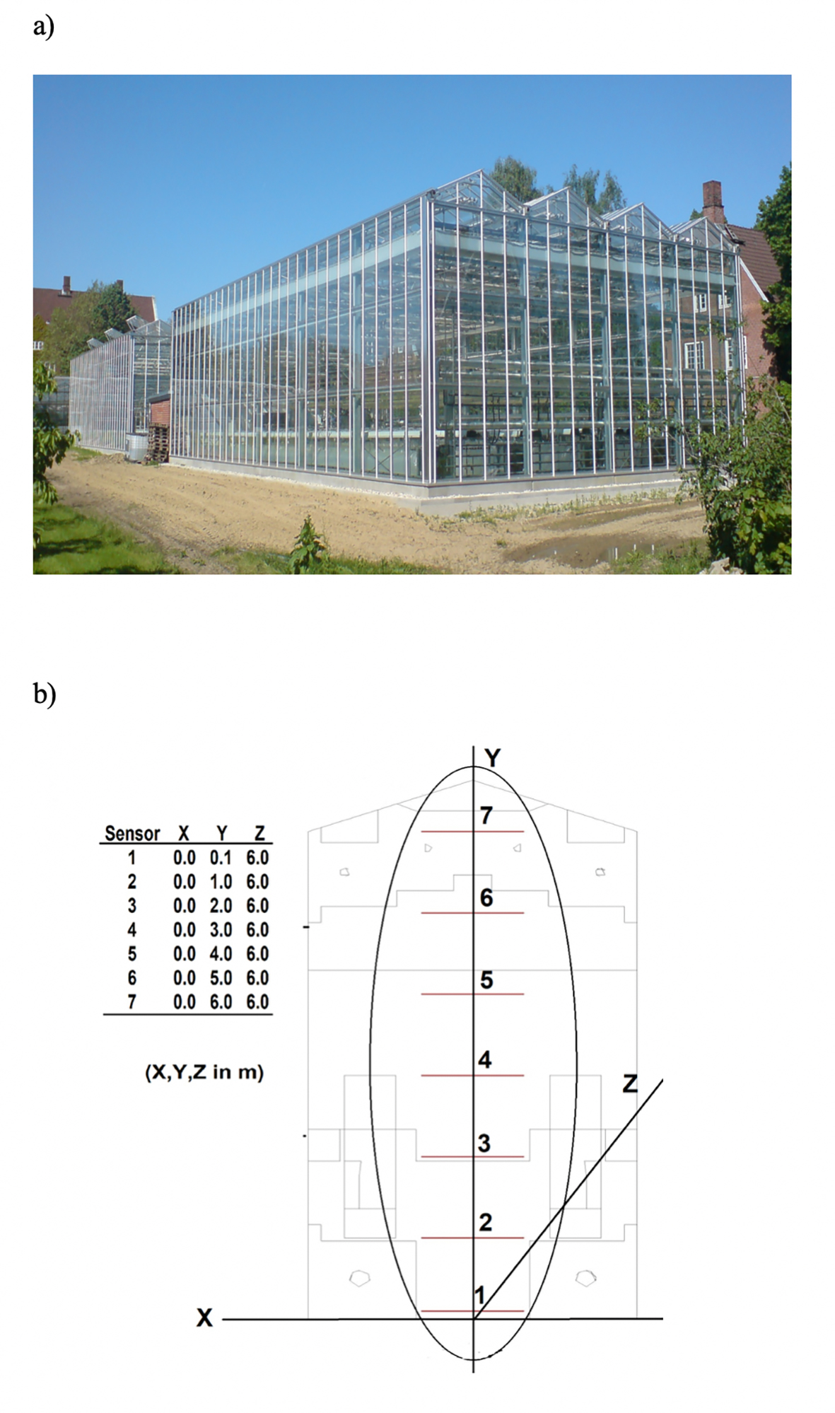
Experiments were conducted in the Department of Biosystems Engineering at the Humboldt University of Berlin, Germany, in a Venlo type glasshouse of four bays. Figure 1a shows the experimental greenhouse and Figure 1b shows the position of the sensors. A tomato crop at full mature stage, with an average height of 3.0 m and a leaf area index (LAI) of 3.0, was growing in the greenhouse during the time of the experiments. Sensors were radiation shielded and placed in the central section of the second bay (from left to right) at heights of 0.1 m, 1.0 m, 2.0 m, 3.0 m, 4.0 m, 5.0 m, and 6.0 m to measure temperature (K) and relative humidity (%) (PTF28, Arthur Grillo, Ratingen, Germany). Wind speed (m s-1) was measured with a hot wire anemometer (Testo 445, Testo AG, Lenzkirch, Germany). There were no physical barriers between the experimental and the other greenhouse bays.
Source: Authors’ own elaboration.
Figure 1 Experimental greenhouse (a) and schematic of one of the greenhouse bays with temperature sensor vertical positions (b).
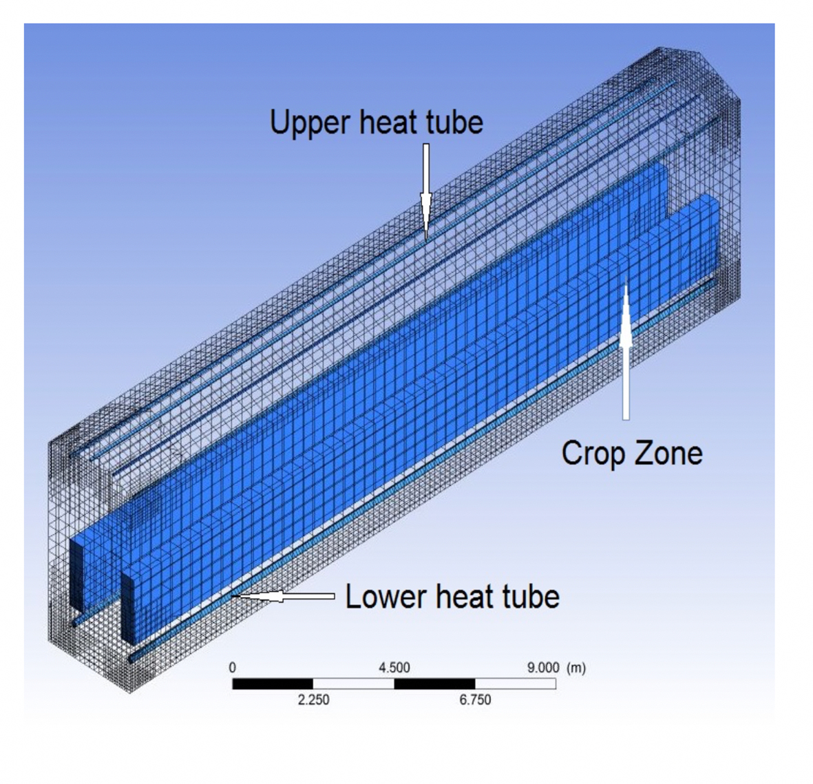
Heating pipes of 0.1 m diameter were positioned along the greenhouse length under each crop line, and additional pipes of 0.05 m diameter were located near the roof in the same direction. The greenhouse had no vents and was fully closed, as shown in Figure 1a. There were no circulation fans in the greenhouse (Figure 2).
Source: Authors’ own elaboration.
Figure 2 Geometry characteristics of the experimental greenhouse bay.
The software Workbench (ver. 14.5, ©ANSYS) was used to create the geometry computational model of the experimental greenhouse bay (Figure 1a). The dimensions of the experimental greenhouse is shown in Table 1. Numerical model and Simulations were run for only one of the bays, where the sensors were placed (Figure 1b). Meshing was built in the module geometry. The dimension of cells was tested until obtaining independence of mesh. The model has a structured mesh with 72 247 nodes and 53 892 elements. The maximum and minimum size of the elements is 0.4 m and 0.1 m, respectively. The left crop has 1263 elements, the right crop has 1217 elements, and the greenhouse has 51 412. The mesh has an Orthogonal Quality of 0.90 and a skewness of 0.02.
The numerical model
The program Fluent (ver. 14.5, ©ANSYS) was used to carry out the simulations by solving the three physical principles that support the Navier Stokes equations: conservation of mass, momentum, and energy. These principles, typically explained by a mass and energy balance on a control volume, can be expressed in a general form by equation 1 (Anderson, 1997).
where ρ is the density of the air (kg m-3), t is time (s), ∇ is the divergence operator (unitless), Γ is the diffusion coefficient, u is the velocity vector (m s-1), and S is the source term. The variable and subscript ϕ represents a dependent variable, which can be mass, velocity, temperature, or a chemical factor, describing the flow characteristics in a location in a specific time point in a three-dimensional space (x, y, z, t). In this study, the source term S ϕ includes the variable ϕ, representing the momentum originated by the drag force produced between the air and the crop. This force could be expressed per unit of volume occupied by the canopy by using equation 2 (Wilson, 1985).
where u is the air velocity (ms-1), L denotes the canopy density (m2m-3), and C D is the drag coefficient, experimentally established by Haxaire (1999) as equal to 0.32. In order to include the effect of friction (drag effect) proportionally to the density of foliage area, the crop was described as a porous media by using the Darcy-Forcchaimer equation (equation 3).
where U is the air velocity (m s-1), µ is the fluid dynamic viscosity (N s m-2), K is the permeability of the porous zone (m2), and C f is the loss coefficient (m-1) assuming a non-linear moment.
In greenhouse ventilation studies, the wind speed is such that the quadratic term of equation 2 dominates over the linear term. This linear term, then, can be neglected due to a small loss coefficient in the non-linear moment equation. The intrinsic permeability K can be deduced combining Equation 2 and Equation 3 by the following relation (equation 4).
Boundary conditions and models used are listed in Table 2.
Table 2 Simulation hypothesis and boundary conditions
| Simulation hypothesis | |
| Solver | Standard SIMPLE, with 3D simulation |
| Formulation | Implicit |
| Time development | State steady |
| Viscosity function | Two equations k-ε Standard (standard wall) and buoyancy model |
| Energy equation | Activated |
| Species model | Species transport: Diffusion energy (vapor h2o) |
| Discrete phase model | Activated |
| Boundary conditions | |
| External wind velocity | Null (adiabatic) |
| Temperature of lower tubes | 303 K |
| Temperature of upper tubes | 283 K |
| Crop simplification | Porous medium |
| Heat source | Constant in the soil, 100 W m-2 |
| Moisture source fraction | 0.012 mass fraction |
| Greenhouse cover | Adiabatic (Heat flux = 0) |
Source: Authors’ own elaboration.
Climate modeling
Air movement is based on a density gradient and, therefore, on the phenomena of convective mass transport. To simulate this phenomenon and include it in the climate modeling, the Boussinesq model, which has proved to be suitable (equation 5) (Boulard, Kittas, Royand & Jafrin, 2002), was used in this study.
where ρ is air density (kg m-3), β is the coefficient of thermal expansion (K-1), T is air temperature (K), and subscript i means initial condition.
Mass diffusion within turbulent flows
Air was assumed as a mixture of vapor and non-consumable gases. In this context, species transport was the model chosen and used for simulations of mass transport, beginning from the diffusion flux of species i, which arises due to gradients of concentration and temperature. Fluent uses the dilute approximation (Fick’s law) to model mass diffusion in a turbulent flow, as written in Equation 6:
where Ji is the diffusion flux of the species i, ρ is the density of the mixture (kg m-3), Di,m is the mass diffusion coefficient (m2 s-1) for species i in the mixture, and DT, i is the turbulent diffusion coefficient (m2 s-1). Yi is the mass fraction of species (kg kg-1) i, and T stands for temperature (K).
For this case, simulations were performed by using a pressure-based solver, the net transport of species at inlets consist of both convection and diffusion. The mass convection component is specified at all the inlets. The diffusion depends on the gradient of the computed species concentration field.
Model validation
The model validation was conducted by setting the boundary conditions listed in Table 2 and by estimating the root mean square error (RMSE) between the measured and estimated values.
Results and Discussion
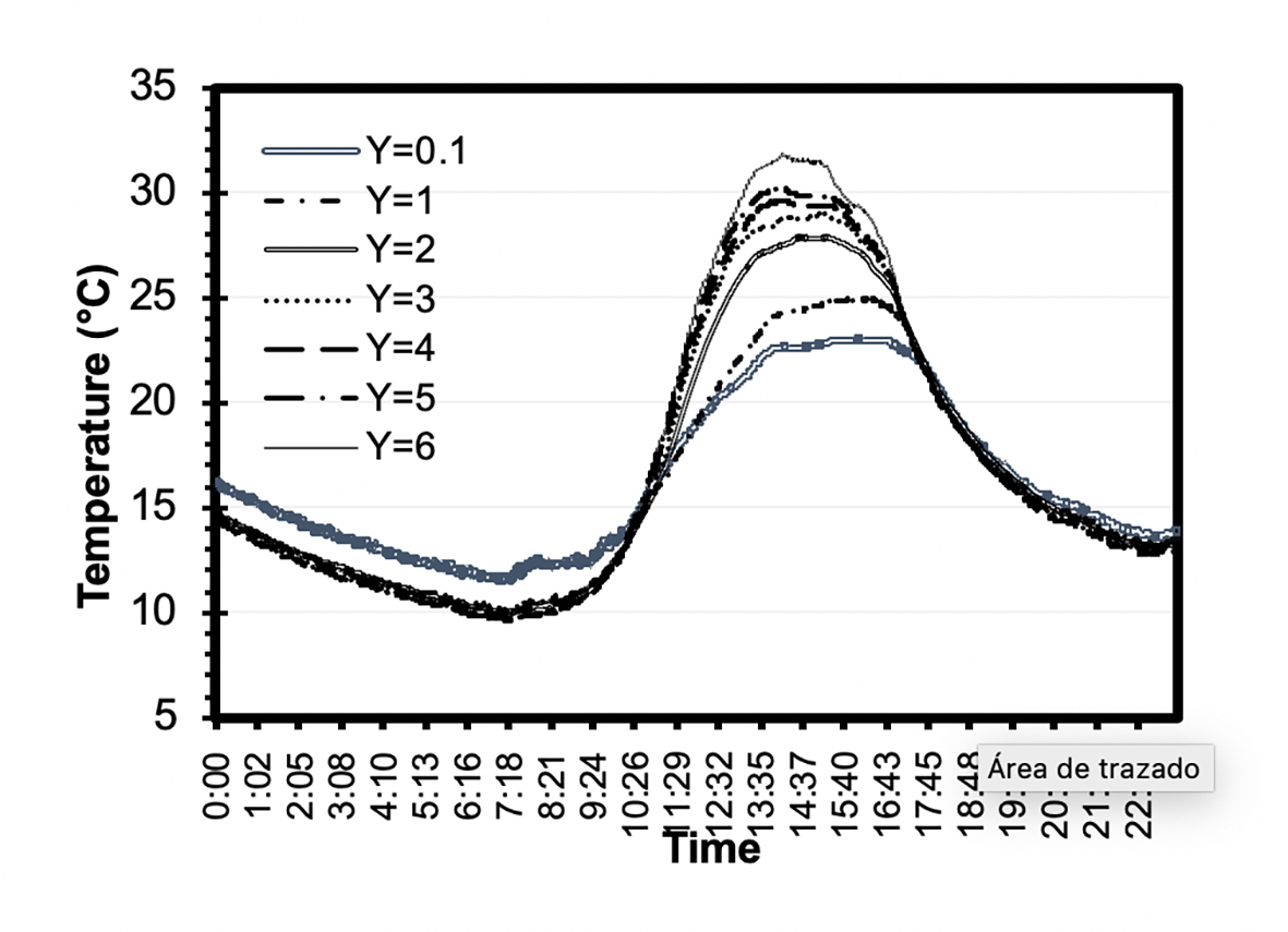
Recorded air temperatures formed thermal gradients of up to 9 K between the lowest and the highest measurement points (Figure 3). All the temperature measurements at different heights followed the same trend, with the readings close to the floor showing the most stable values. Air temperature was driven principally by the heat accumulated due to the incident solar radiation. Figure 3 shows how both variables, radiation and temperature, have the same behavior, with the temperature showing a time delay. Similar findings have been reported by other authors (Popovski, 1986; Teitel & Tanny, 1998). Temperature measurements on lower heights tended to be more stable, indicating that the canopy may be acting as a buffer between the soil and the portion of greenhouse air located above the canopy. During night, thermal gradients did not exceed 3 K.
Source: Authors’ own elaboration.
Figure 3 Experimental data air temperature (°C) in the experimental greenhouse bay at 0.1 m (-), 1.0 m (+), 2.0 m (X), 3.0 m (Δ), 4.0 m (◊), 5.0 m (○), and 6.0 m (□) of height.
In contrast, the maximum temperature differences in the vertical direction were registered around 15:00 h. The greatest temperature gradient (5 K) occurred between the soil and the top of the canopy (0.1 m-2 m height). The rest of the temperature gradient (4 K) was distributed from 2 m to 6 m of height. The minimum temperature differences among heights were registered at around 11:00 h and at around 18:00 h. These times are when inversions of temperature occurred between the air at heights near the ground surface and the air at heights close to the roof.
All the results indicate that the greenhouse air temperature lowered to undesired values (<283 K) for plant production before sunrise. Even though the integrated temperature for the 24 h period was 289.75 K, it is still not desirable to have temperatures of 283 K in the greenhouse. Plants integrate temperature, but they make it under a reasonable range, and 283 K may be outside of such range. Brun & Lagier (1985) consider night temperatures of 285 K-288 K as appropriate, while Williams (1973) recommended 286 K. Moreover, Calvert & Slack (1975) suggested 293/291 K as the optimum day/night temperatures.
The thermal differences between day and night are also important, and temperatures of 6 K-7 K between maximum and minimum temperatures during a 24 h period are optimum for tomato (Went, 1944). Therefore, the presence of temperatures as low as 283 K and as high as 305 K (Figure 3) may not be adequate for a tomato crop.
The low temperatures registered before sunrise also suggest that the energy trapped in the soil during the previous day, and released during the night, was not enough to keep the greenhouse atmosphere within appropriate conditions for plant growth. Thus, this greenhouse is in need of a heating system to operate during a portion of the day to avoid low values and high variations of temperature. The climate behavior under such scenario, which includes a heating system, was assessed through simulations by using CFD.
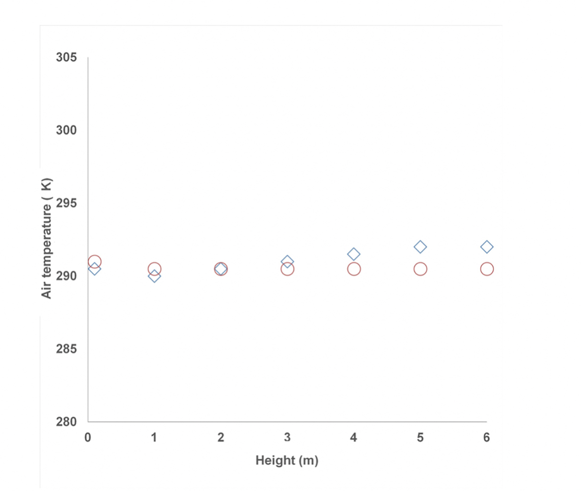
During the validation process, values of inside air temperature showed a good agreement, with a RMSE between the measured and the simulated air temperatures equal to 1.61 K, evaluated at seven different heights in the center section of the experimental bay (Figure 4). Such validation results indicate that the model has a reliable accuracy for the application intended for this study.
Source: Author’s own elaboration.
Figure 4 Statistical valuation (RMSE) of model between measured (◊) and simulated (○) values of air temperature (K) at seven different heights in the center section of the greenhouse bay.
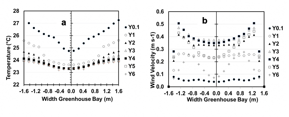
After validation, simulations were run to evaluate the air dynamics and the temperature behavior for the closed greenhouse during the operation of the heating system. Results indicate a convective flow from the center of the greenhouse bay to the walls, with a pronounced temperature gradient close to the soil (Figure 5a). Even if the wind speeds are low (Figure 5b), temperatures are non-uniform (Figure 5a).
Source: Authors’ own elaboration.
Figure 5 Simulated (a) air temperature (K) and (b) wind velocity (m s-1) at different levels of the experimental greenhouse bay. Centered line (Y) denotes height in meters.
In the area close to the ground, wind speeds do not surpass 0.1 m s-1 (Figure 5b) and the air comes from the center (hot zone) to the walls (cold zone). While the energy has to be sustained by the heating system, the airflow is directed to the roof where wind speeds of 0.3 m s-1-0.5 m s-1 can be observed at heights of 4 m-5 m. Wind velocities were more unstable near the roof compared to wind velocities at lower heights. In this zone, the airflow might be more turbulent that at lower heights due to the proximity to the heating pipes.
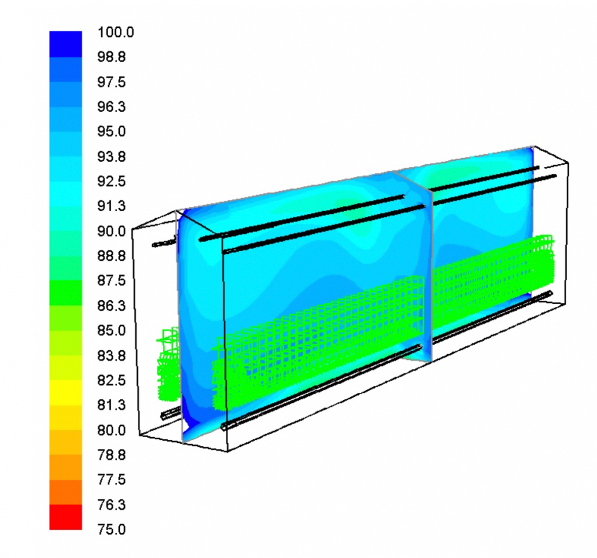
The presence of plants also affected the air temperatures because of the high moisture levels produced within the greenhouse, especially around the crop zone (Figure 6), with only small humidity gradients generated within the canopy. With a closed greenhouse, plant transpiration caused high rates of condensation during the night (data not shown). The previous results highlight the need to use the heating system not only for temperature control but also for humidity control, given the restricted air movement conditions prevailing in the greenhouse.
Source: Authors’ own elaboration.
Figure 6 Longitudinal profiles of simulated relative humidity (%) at the center section of the greenhouse bay.
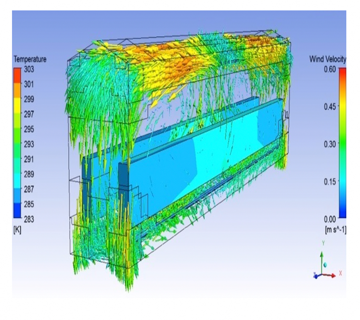
Figure 7 shows the wind dynamics inside the bay, and the temperature within the crop zone. Even though the crop is only a porous zone, both the heat stored in the floor and the heat pipe tube resulted effective to heat the plants from the center of the framework and from the roof.
Source: Authors’ own elaboration.
Figure 7 Contour of simulated crop temperature (K) and wind velocity vectors (m s-1) inside the greenhouse bay.
From two-dimensional scenarios previously simulated by Rojano et al. (2013), it was found that the vertical ascending heat flow was due to the buoyancy term. The air internal motion was then described and predicted by using the transient and the convective forces, terms given by the strong dependency of air density as a function of temperature.
As indicated in Figure 3, the energy from radiation trapped in the soil was not sufficient to keep the greenhouse warm a day round. Thus, supplemental energy had to be provided by the pipe heating system, above all in the night (Montero et al., 2013). If additional energy would have been stored and then released from the soil, the operation of the heating system would have not been required.
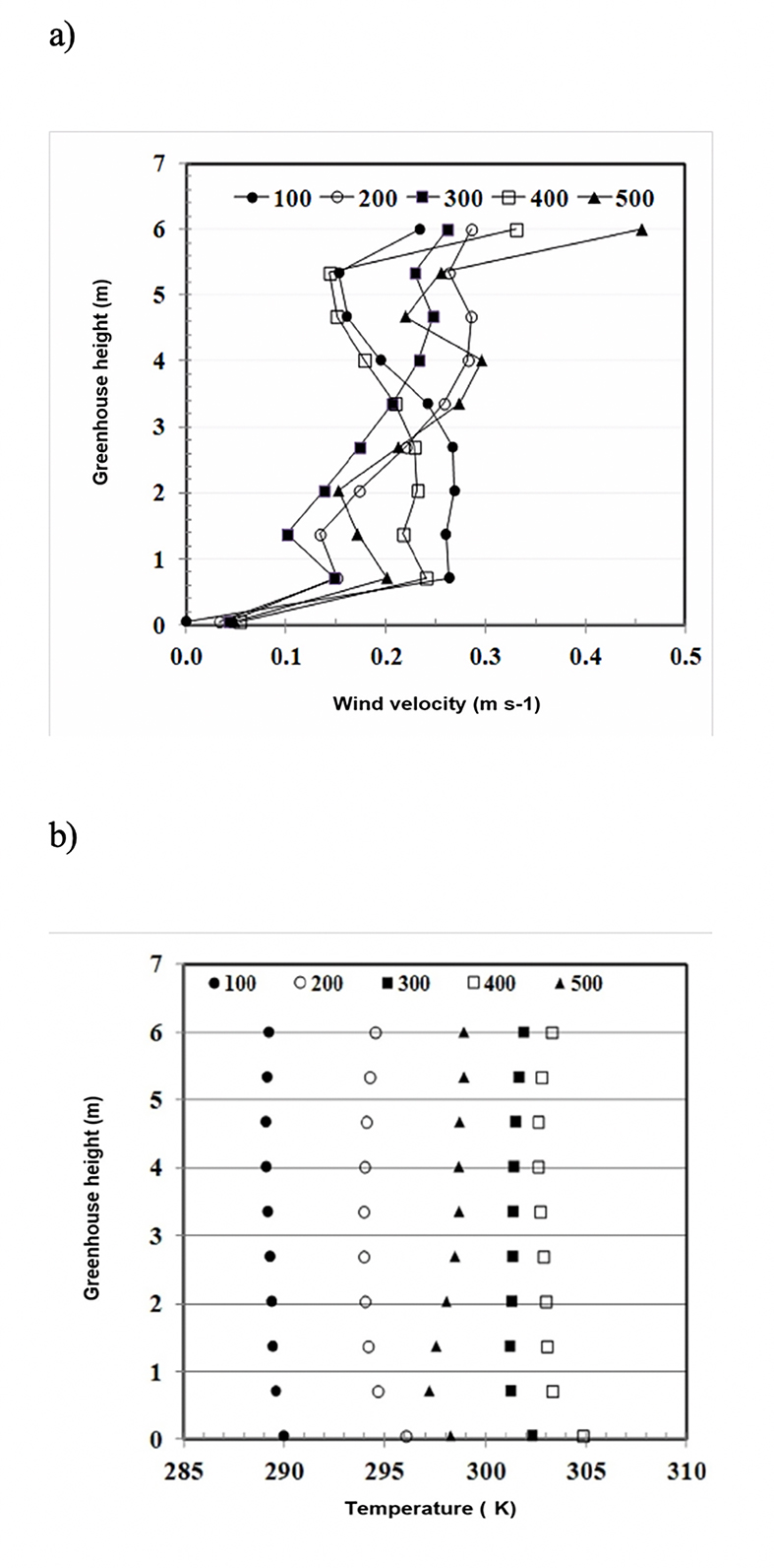
Based on the above, and to find out what amount of energy released from the soil would be necessary to keep appropriate conditions within the greenhouse, several magnitudes of energy as sensible heat from the soil were simulated (Figure 8). Results showed that air temperatures produced in the vertical profile were uniform (Figure 8b). Along with the air temperature, wind velocities (Figure 8a) also presented in general uniform distributions. From Figure 8b, it could be seen that a heat flux of 200 W m-2 would produce adequate inside air temperatures of around 294 K. Such value of air temperature inside the greenhouse is desirable for vegetable production. This highlights the need for future research on the use of thermal efficient materials for an enhanced energy collection on the floor and reduction of heating costs.
Source: Authors’ own elaboration.
Figure 8 Scalar values of (a) wind velocity (m s-1) and (b) air temperature (K) inside the greenhouse, with simulation of seven heat flux sources (W m-2) from the soil surface.
Figure 8b shows how the air temperature did not increase linearly by increasing the amount of heat provided to the greenhouse from the soil. Under the experimented conditions, the energy transferred by convection needs air in order to propagate. In this case, the amount of air available for energy transport was limited and, in consequence, air temperature did not increase for the case of 500 W m-2. Reported by several authors, heating systems in greenhouses is an important sink of energy in the crop production cycle (Bazgaou et al., 2018; Gourdo, Fatnassi, Bouharround, Ezzaerj & Bazgaou, 2019). Temperature differences between the pipes located at the ground and roof levels could keep increasing; however, that would did not produce more momentum, and the energy exchanged by convection reached its maximum and then tended to decrease.
Conclusions
Environmental data measured inside the greenhouse showed that heat, built up in the soil due to solar radiation, keeps the environment within the tomato comfort zone for several hours during the day, mainly from noon to evening. However, heat lost by long-wave radiation at night caused inversion. Applying heat artificially through pipes placed underneath the crop zone promoted uniform distribution of temperature within the plant canopy. With that system, uniform distributions of wind velocity and humidity were also promoted.
A heat flux of 200 W m-2 simulated from the ground would produce inside air temperatures of 294 K, which is desirable for vegetable production, thus, highlighting the necessity of using thermal efficient materials in the ground covers to enhance energy collection and contribute to reduce heating costs under closed greenhouse conditions.
An increment of the simulated heat released from the soil to values greater than 400 W m-2 did not promote a linear increment of the greenhouse air temperature, suggesting that appropriate conditions did not exist to promote air movement, and the energy exchanged by convection reached its maximum and then decreased. In order to favor the energy transfer by convection, there must be air to be removed. Compared to an open greenhouse under closed conditions, there exists a deficit of air for energy transport.
Results showed the behavior of the greenhouse environment as regulated by natural convection when assisted by a pipe heating system. This information may be useful in Mexican greenhouses under specific climate conditions.

