


 nueva página del texto (beta)
 Inglés (pdf)
 Artículo en XML
 Referencias del artículo
 Enviar artículo por email
 Citado por SciELO
  Similares en
SciELO
Similares en
SciELO 
 Permalink
Introduction
In addition to its theoretical interest, it is well known that Dawson’s integral (or Dawson’s function) arises naturally in several physical applications, whereby the research related to this function is relevant. In this context, heat conduction problems (Briozzo & Tarzia, 2010; Petrova, Domingo, Tarzia & Turner, 1994) (see section 5), theory of electrical oscillations (McCabe, 1974; Weisstein, 2017), relativistic hydrodynamics (Scott, 2007), chemical physics in birefringence and dielectric relaxation phenomena in presence of strong electric fields (Prigogine & Rice, 2001), among many others, are mentioned.
The aim of this article is to propose a handy invertible and integrable approximation
for Dawson’s function. In the literature, there are several Dawson’s function
approximations reported; for instance, Sykora
(2012) proposed various approximation orders with good accuracy, although
they are not sufficiently simple nor are they hardly invertible and integrable.
Moreover, Boyd (2008) proposed an accurate
approximation for Dawson’s integral, by solving its differential equation using the
orthogonal rational Chebyshev functions of the second kind; nevertheless, its
rational approximation is hardly invertible and integrable. In the same way, Cody, Kathleen & Thacher (1970) proposed
rational approximations for Dawson’s integral, although the accuracy of the reported
results was verified only in finite intervals and not in the total domain of
Dawson’s function. Lether (1997) developed a
family of rational functions for computing Dawson's integral. Although this work got
approximations with a low relative error, its expressions are too large to be
invertible and integrable. Lether (1998) investigated the relation between some
rapidly convergent series of exponential functions for computing Dawson's integral.
Since the approximation is given in terms of an infinite sum of terms of the form
An example of the importance of inverting the Dawson’s integral is mentioned by Scott (2007). In this work on relativistic hydrodynamics, the time (t) measured by a reference observer is expressed in terms of a scale factor (r), which determines the shape of an entropy profile through Dawson’s function. His work mentions that in order to complement the solution of the problem in this part, it is necessary to invert the mentioned expression in order to obtain r as function of t, and, thus, obtain the velocity gradient. This work targets this kind of applications.
In fact, the subject of inverting and approximating the integral for Dawson’s function is little addressed in the literature and this will be the main goal of this work.
The rest of this paper is organized as follows. In Section 2, the basic idea of the power series extender method (PSEM) (Vazquez-Leal & Sarmiento-Reyes, 2015), which plays an important role in this work, is introduced. Section 3 will provide a brief introduction to Dawson’s integral. In Section 4, the deduction of a handy, accurate, invertible and integrable expression for Dawson’s function is provided. Section 5 proposes an application of Dawson’s integral to a non-classical Stefan problem in physics. Section 6 discusses the main results obtained and includes a table for the benefit of the readers with the relevant contributions found in this work. Section 7 provides a brief conclusion and, finally, Section 8 resumes some results of cubic algebraic equations relevant for this work.
Basic Concept of PSEM method
Here it is assumed the case of nonlinear differential equations, expressed in the form
with a boundary condition given by
L and N are linear and nonlinear operators, respectively, f(x) is a known analytic function, B is a boundary operator, Γ is the boundary of domain Ω and ∂u/∂η denotes differentiation along the normal drawn outwards from Ω (Cody et al., 1970).
In accordance with the PSEM methodology (Vazquez-Leal & Sarmiento-Reyes, 2015), the solution of (1) is expressed as a power series
Where v k (k = 0,1,2,…) denotes the coefficients of the power series.
It should be mentioned that there is no single way of obtaining (3); thus, some approximate methods from the literature could be employed for that purpose such as Homotopy Peturbation Method (HPM), Homotopy analysis method (HAM), Variational Iteration Method (VIM), Differential Transform Method (DTM), Adomian Decomposition Method (ADM), Taylor Series Method (TSM), and Power Series Method (PSM), among others (Vazquez-Leal, Castañeda-Sheissa, Filobello-Niño, Sarmiento-Reyes & Sánchez-Orea, 2012). Next, following the PSEM method, it is proposed that the solution for (1) can be written as a finite sum of functions in the general form
or
(Vazquez-Leal & Sarmiento-Reyes, 2015), where u i are constants to be determined by PSEM, f i (x,u i ) are in principle arbitrary trial functions; and n and 2 n denote the orders of approximations (4) and (5), respectively. It is agreed to denominate (4) and (5), from here on, as the trial function (TF). Next, the Taylor series of (4) and (5) is calculated, resulting in the power series
respectively, where Taylor coefficients P k are expressed in terms of parameters u i .
After equating/matching the coefficients of power series (6) or (7) with those corresponding to (3), the values of u i are obtained. Finally, by substituting them into (4) or (5), it is obtained the PSEM approximation. It is important to note that (4) or (5) can separately be applied to obtain an approximate solution of (1). As a matter of fact, the selection of TF depends on the nature of the problem under study. In addition, it is important to remark that if the f i functions are chosen to be analytic, then (6) and (7) are convergent series (Belser, 1999; Oberguggenberger & Ostermann, 2011; Zill, 2012).
Some rudiments of Dawson’s integral
Dawson’s integral is defined by Khan (1990) as
As a matter of fact, it is not difficult to prove that F(x) satisfies the following initial condition problem:
On one hand, assuming a power-series expansion of the form
On the other hand, it is possible to show that, after integrating by parts and employing a breakpoint, F(x) is properly expressed by the following asymptotic expansion for large values of x (Khan, 1990).
Nevertheless, it will be exposed a notable fact that it is possible to use (11), keeping just the first two terms of the series to represent F(x), even for relatively small values of x with good accuracy, in order to get a handy approximation, valid for x ≥ 0 (see Section 4).
The function F(x) has just one extreme value, a maximum that is x=0.923 where F adopts the value F(0.923)=0.5410435224
Deduction of a handy accurate invertible and integrable expression for Dawson’s function
With the purpose of obtaining an approximated expression for Dawson’s function, an algorithm will be followed by dividing the domain of F(x) into two. In the first subinterval, Dawson’s integral will be modeled by using the PSEM method, while in the second one, it will be shown that employing the first two terms of (11) in order to obtain a good approximation is sufficient.
To begin, equation (10) is used to obtain the following expression for Dawson’s integral F(x), valid for values near the origin:
In accordance with the PSEM algorithm (Vazquez-Leal & Sarmiento-Reyes, 2015), it is proposed to model the first part of F(x) near the origin by means of the following rational function (see (5)):
Where b1, b2, ɑ1, ɑ2, and ɑ3 are parameters to be adequately determined later on.
The following expression shows some terms of the Taylor series of (13):
Next, a system of algebraic equations will be deduced to calculate the values of the parameters mentioned above through the following criteria.
In order to ensure that r(x) correctly represents the behavior of F(x) for values near the origin, the Taylor series (12) and (14) will be matched by equating the coefficients of powers x and x 2. Since there are five parameters to be determined, then three additional equations are necessary, chosen so that the proposed rational function describes points of F(x) farther from the origin.
With that purpose, the following points of Dawson’s function are proposed: A(0.923,0.5410435224), B(1.5,0.4282490711), and C(2.5,0.2230837222) (it is noted that A corresponds to the point where F(x) reaches its extreme value (see section 3)).
The algebraic system of equations emanating from the above considerations is the following:
The numerical solution for the above system is
After substituting (16) into (13), it is obtained
As it can be seen afterwards, (17) describes F(x) adequately for values of x, from the origin to x≈2.6789.
For x greater than this value, it is proposed to model F(x) with the first two terms of expansion (11), that is,
It will be seen that, despite the character asymptotic of (18), A(x) describes with good precision Dawson’s function in the mentioned interval (Figure 1 and Figure 2). It is emphasized that although a better approximation for r(x) may be obtained, assuming a rational function of greater order (see (13)) and increasing the accuracy of A(x) keeping more terms of (11), the goal is to obtain an accurate expression, as simple as possible, for Dawson’s function, in such a way that it is invertible and integrable. As a matter of fact, as an application, this last characteristic of this approximation for F(x) will be employed in a case study emanating from physics. On the other hand, in order to build a continuous function from (17) and (18) it is necessary to find the point of junction of the previous functions. The fact that the absolute values of relative errors of (17) and (18) have to be the same in the point of intersection of r(x) and A(x), i.e., is proposed as criteria:
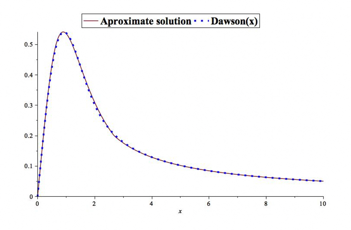
Source: Author’s own elaboration.
Figure 1 Plots of proposed approximation (22) and numerical Dawson's function.
After applying condition (19), the value already mentioned is obtained:
In a sequence, by using the unit step function δ (Zill, 2012), it is possible to express (21) as
(Figure 1).
Next, it is noted that (21) is indeed invertible.
For the interval x>2.678915610, F(x) is given by (18), in such a way that after some algebraic steps, (18) is rewritten as
where, for the sake of simplicity, the dependence of x from A(x) is omitted.
In Appendix A the basic aspects of cubic algebraic equations are summarized.
Next, Q, R, and D are calculated (see equations (A1) and (A2)) so that
Since discriminant D>0 for the whole interval x>2.678915610, it is inferred that (23) has just one real root which, in accordance with the first equation of (A3), is given by
after using F(x) instead of A(x).
On the other hand, for the interval 0≤x≤2.678915610, F(x) is given by (17):
After some algebraic steps, (17) is rewritten in the form of the cubic equation
where F(x) has been employed instead of r(x) and defined
The corresponding values for Q and R are given by (see A [2])
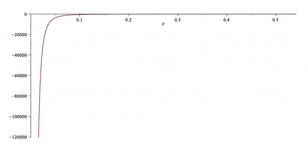
On the other hand, in order to obtain D, it is just necessary to substitute (28) and (29) into
nevertheless, a sort of cumbersome expression to D would be obtained.
A better methodology is to graph the right-hand side of (30) (see Figure 3). From the mentioned Figure, it is concluded that, D>0 in the interval of interest 0<x≤2.678915610 and from the theory for solving cubic equations, (26) provides three real roots (see Appendix A).
Next, from the three above-mentioned roots, the last expression x 3 of (A4) is provided as a solution for (26), because this supplies, with good precision, the values of x, starting from the values of Dawson’s function F:
for the interval 0<x≤2.678915610
Finally, it is noted that the approximation proposed to Dawson’s integral (21) is also integrable, in terms of elementary functions, that is to say,
(for real arguments x, y, the two-argument function arctan(y,x) computes the principal value of the argument of the complex number x+iy, so (π<arctan(y,x)≤π. Equation (32) was obtained with the assistance of Maple 17 built-in function routine for integration.
In terms of step function, it is possible to rewrite (32) as
where the value 0.97010971726 expressed in the interval x>2.678915610
represents the value of
In order to prove the accuracy of (33), regarding the relevant contribution that comes from 0≤x≤2.678915610, the area will be evaluated:
and later it is compared with the numerical value of (34) for Dawson’s function. As a matter of fact, the accuracy of the proposed approximate solution (33) is revealed.
The numerical value of (34) turns out to be 0.9635924825, while the value
obtained after employing the proposed analytical approximation (33) is
0.9701971726. What is more, Figure 4 shows
the plot of the area function
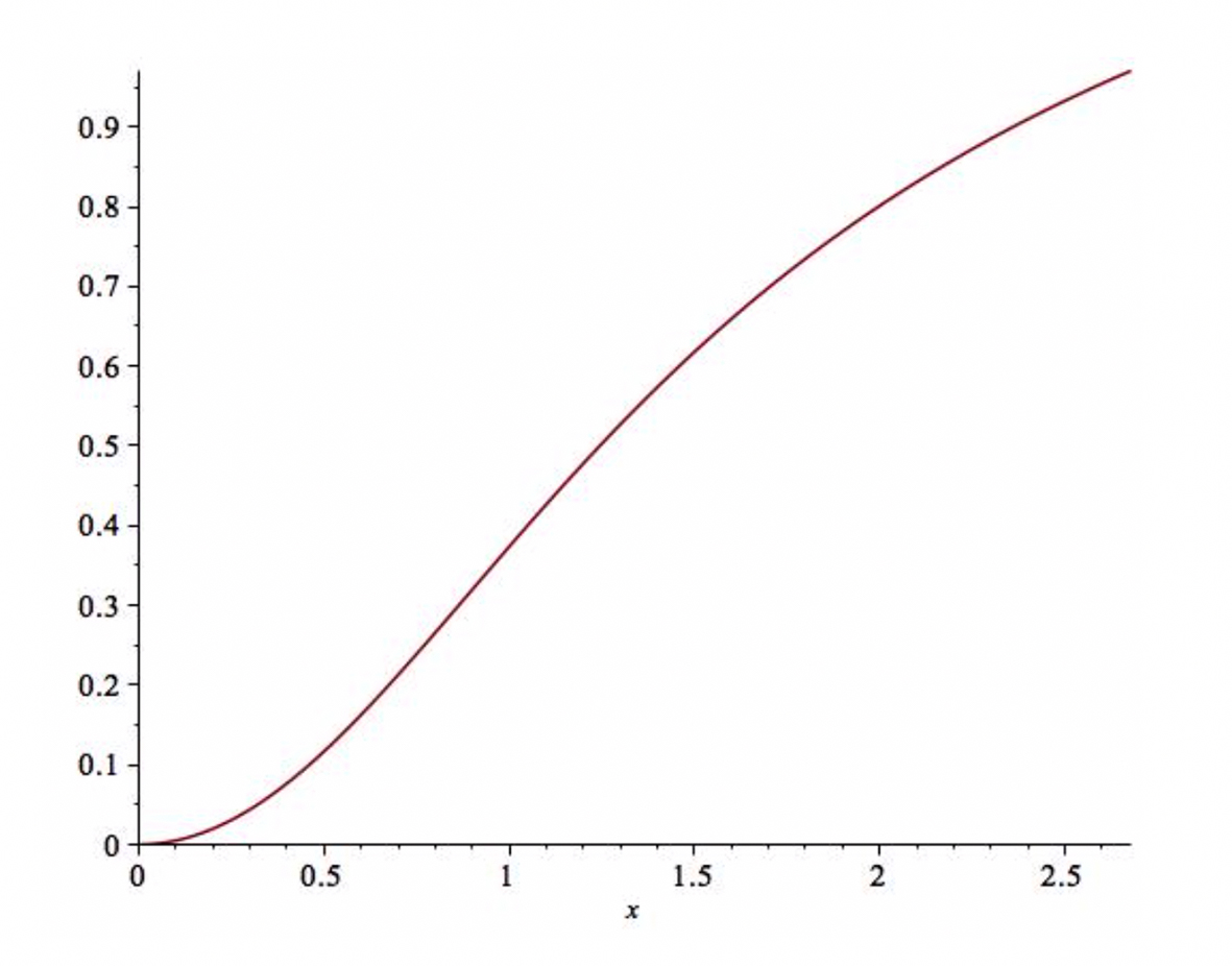
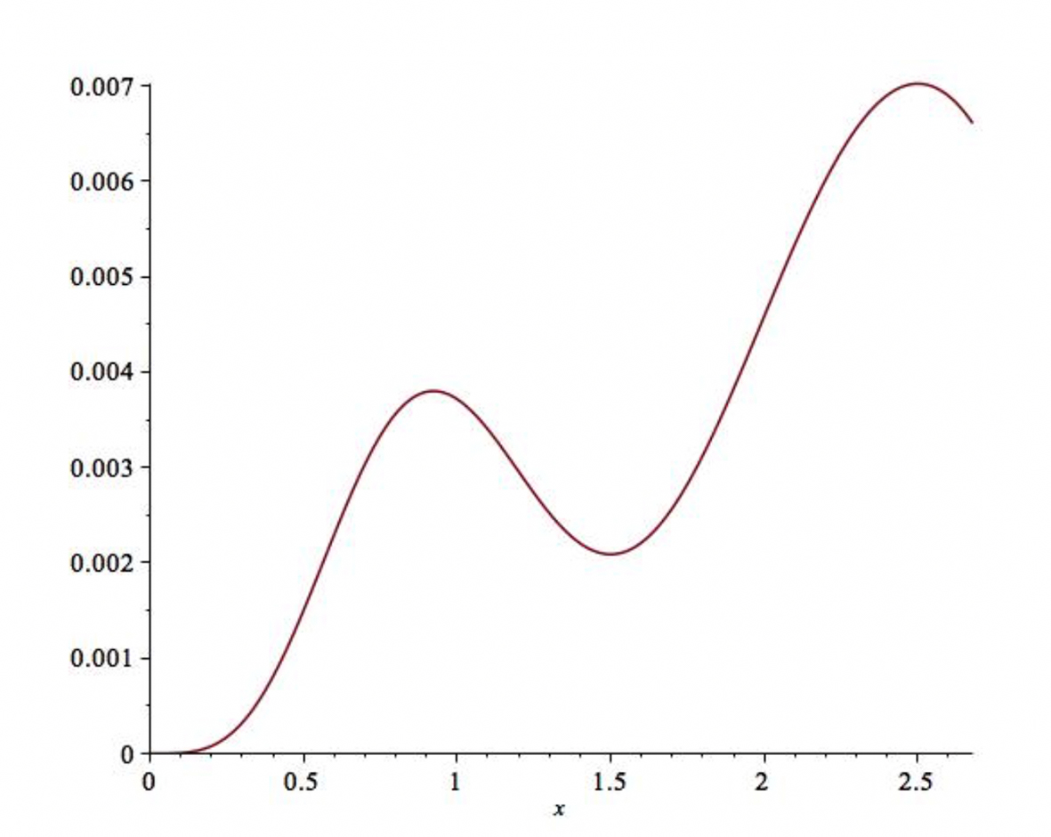
Source: Authors’ own elaboration.
Figure 4 Plot for the area function
Application to a nonclassical Stefan problem in physics
A one-phase Stefan problem for a semi-infinite material is a free boundary problem for the heat equation, which aims to find the temperature distribution for the case of melting and solid phases, as well as to determine the evolution of the free boundary.
Following Briozzo & Tarzia, 2010, it is briefly considered the nonclassical heat conduction problem for a semi-infinite material given by the conditions
where u=u(x,t) is the temperature, x=s(t) is a free boundary, k, ρ, C, l, and γ are certain positive thermal coefficients, the boundary temperature is denoted by f>0, and λ 0 is a constant. With the purpose of getting an explicit solution of a similarity type, the following substitution is proposed (Briozzo & Tarzia, 2010):
where ɑ2=k/ρc is the diffusion coefficient of the phase change material.
After using (36), it can be noted that (35) adopts the form
where the dimensionless parameter
has been defined, and s(t) must be of the form
The value of the parameter η 0 is determined later.
From Briozzo & Tarzia (2010), the solution of (37) that satisfies the conditions (38) and (39) is given by
where the following is defined:
In (44), erf(x) denotes the error function
and F(x) the Dawson’s integral (see (8)).
By substituting (43) and (44) into (40), it is obtained the following equation for the unknown parameter η 0 (Briozzo & Tarzia, 2010):
where the Stefan’s number given by Ste=fc/l>0. has been introduced.
It is noted that one of the main contributions of this work is to provide an analytical approximation for the integral of Dawson's function (see (33)) with good precision and, for the same reason, this result may be employed into (44). On the other hand, Vazquez-Leal, Castañeda-Sheissa, Filobello-Niño, Sarmiento-Reyes & Sanchez-Orea (2012) provided the following handy accurate analytical approximation to the error function erf(x) (see discussion):
Thus, unlike Briozzo & Tarzia (2010), who just provided a symbolic solution to problems (37)-(40), the authors in this study are in a position to propose an analytical solution for the same problem with good precision by substituting (33) and (47) into (43).
Finally, approximations (22), (33) and (47) may be substituted into (46) in order to obtain a numerical approximate solution for η 0 and, with this result, the problem is concluded.
For sake of simplicity, the following values of Stefan’s number Ste=1 and λ=1 are proposed as a case study. After performing the numerical solution of the above-mentioned equation, the value η 0=1.479186840. is obtained.
Discussion
This article successfully accomplished the purpose originally proposed: to get a handy analytical approximate solution for the Dawson’s integral, which, as seen before, describes for example the solution of heat conduction problems (Briozzo & Tarzia, 2010; Khan, 1990). Although the proposed approximation has an acceptable precision, it introduces two advantageous characteristics, which are not presented in other approximations of Dawson’s function from the literature: being invertible and integrable in terms of elementary functions. To achieve this goal, a piece wise-like approximation was proposed, for which the interval of definition [0,∞) is divided into two subintervals: [0,2.678915610] and (2.678915610,∞).
For the case of [0,2.678915610] it was required the application of the PSEM method (Vazquez-Leal & Sarmiento-Reyes, 2015) in order to adequately model Dawson’s function in this interval. Such as it was explained in Section 4, it was proposed to model Dawson’s function near to the origin by means of the rational function (13), provided with five parameters to be determined. Next, a system of algebraic equations was deduced to calculate the above mentioned parameters, first, by equating the coefficients of powers x and x 2 from Taylor series of the proposed solution (14) and the expansion for Dawson’s integral (12), valid for x values near the origin. In order to obtain three additional equations, the points denominated as A, B, and C into (13) were substituted. After solving the resulting system of equations (15), it was obtained (17). It is emphasized that the procedure mentioned ensures that (44) describes adequately and with good precision Dawson's function for xvalues from the origin to 2.678915610. With the purpose to model Dawson’s function for the interval x>2.678915610, the first two terms of its asymptotic expansion (11) were kept (see (18)). It is remarkable the accuracy with which the above mentioned truncated asymptotic expression of only two terms (18) describes Dawson’s integral, starting from relatively small values of x, in absolute value. Although a better approximation for r(x) may be obtained, regarding a rational function of a greater order than five and increasing the accuracy for values x>2.678915610, considering even more terms for the truncated series (18), the goal of this research was to obtain an approximation, as simple as can be, to get an invertible and integrable Dawson’s analytical approximation.
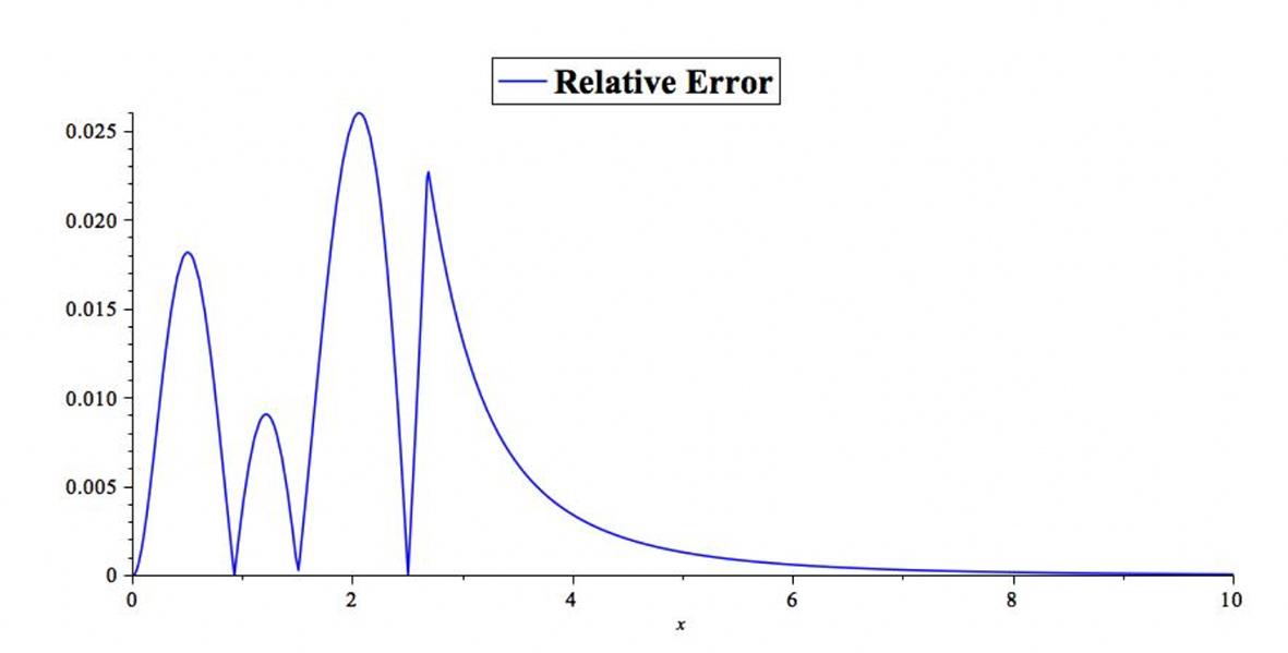
Thus, from the above discussion it was natural the proposal of a piece-wise approximation of the form (22), where the step function in order to get a compact expression for F(x) was employed. Although from Figure 1 it is clear the accuracy of the proposed approximation (22), Figure 2 shows that the biggest relative error committed employing (22) is about 2.5%, from which it can be inferred that the proposal in this research provides a good precision. As a matter of fact, the possibility of providing an invertible and integrable Dawson’s analytical approximation is indeed complicated to obtain, and it was noted that (22) indeed turns out to have both characteristics.
For the interval x≥2.678915610, F(x) is given by (18). After carrying out some algebraic steps, it was possible to express (18) in terms of cubic equation (23), and from Appendix A, it was concluded that (23) just owns one real root, because D>0 and it is given by (25). On the other hand, for 0≤x≤2.678915610, (17) is rewritten in the form (26). After taking into account the results of Appendix A, it was concluded that (26) provides three real roots (because D is negative for all values of x in the interval), and the root that better describes the values of x, in terms of values of the Dawson’s function, is given by (31). It was noted that instead of calculating the value of D directly, the novel procedure of plotting the right hand side of (30) was chosen (Figure 3) with the result mentioned above. Once again, it is emphasized that handiness of (17) and (18) allowed to get an invertible expression for Dawson’s integral.
Next, it is noted that our approximation to Dawson’s integral (21) is also integrable, in terms of elementary functions through the remarkable results (32) or (33). In order to prove the accuracy of the relevant contribution of (33) that comes from the interval 0≤x≤2.678915610, it was considered to evaluate the area integral (34) employing (33), and the resulting value was compared with the numerical value of (34). The numerical value of (34) turned out to be 0.9635924825, while the value obtained after employing the proposed analytical approximation (33) was 0.9701971726. In a sequence, Figure 5 shows that the biggest absolute error committed is about 7×10⁻³, from which it is deduced the accuracy of approximation proposed here.
Finally, in order to show the usefulness of the results presented in this work, the case of a one-phase Stefan problem for a semi-infinite material was introduced. These problems involve the heat equation, which aims to find the temperature distribution for the case of melting and solid phases, as well as to determine the evolution of the free boundary (Briozzo & Tarzia, 2010).
The procedure proposed by Briozzo & Tarzia
(2010) express the original non-classical heat conduction problem for a
semi-infinite material (35), in terms of the ordinary differential equation (37),
which obeys the conditions (38)-(40), through substitutions (36). Following Briozzo
& Tarzia (2010), the solution of (37) that satisfies the conditions (38) and
(39) is given by (43). It is remarkable that (43) is expressed in terms of integrals
of Dawson's function and error function. It is noted that the integral of the
Dawson's function can be expressed in terms of the generalized hypergeometric
function
As it was already mentioned, the value obtained after employing the proposed analytical approximation (33) was 0.9701971726, and the corresponding absolute error committed by using (32) was only 7×10⁻³ (Figure 5). Thus, it is concluded that our proposed approximation has a good precision and it is expressed in terms of elementary functions.
On the other hand, Vazquez-Leal et al. (2012) provided a handy accurate analytical approximate solution for the error function erf(x) (47). The mentioned article compares different approximations for the error function presented in the literature. From them, (47) turned out to have a relative error lower than 2×10⁻⁴, and for the cumulative error function, the maximum committed error for region x>0 is lower than 9×10⁻⁵. Therefore, (47) has a high level of accuracy, comparable to other approximations found in the literature; nevertheless, the proposed approximation has such mathematical simplicity that allows to be used on practical engineering applications and sciences with good precision. Thus, unlike Briozzo & Tarzia (2010) who just provides a symbolic solution to problem (37)-(40), an analytical approximate solution was provided for the same problem and, from the above mentioned, with good precision by using (33) and (47) approximations into (43).
Finally, with the purpose of completing the solution to the proposed problem, approximations (22), (33), and (47) were substituted into (46) in order to obtain a numerical approximate solution for η 0. As a case study, it was proposed the following values of Stefan’s number: Ste=1 and λ=1. The numerical solution of the above-mentioned equation provided the value η 0=1.479186840.
Next, a table is provided with the relevant contributions found in this work.
Proposed approximation to Dawson’s Function:
Proposed approximation to Inverse Dawson’s Function:
Proposed Integral for Dawson’s Function in Terms of Elementary Functions:
Conclusions
This work proposed a novel analytical approximation for Dawson’s function in the form of a piecewise type function (22). Given the different nature of F(x) for values of x close to the origin and far from it, it is natural to propose a solution by sections. Nevertheless, it is emphasized that although a better approximation for Dawson’s function may be obtained, assuming a rational function of greater order (see (13)) and increasing the accuracy of A(x) (see (18)), keeping more terms of series (11), the goal of this study was to obtain an accurate expression as simple as possible, in order to get an invertible and integrable F(x) function with good precision. To achieve this goal, the domain of this study was divided into two intervals: [0,2.678915610] and (2.678915610,∞).
With the purpose of modeling F(x) in [0,2.678915610], the PSEM method was used (Vazquez-Leal & Sarmiento-Reyes, 2015), whose methodology required to employ three known points of Dawson’s integral in order to propose a rational approximation provided with five parameters, which were successfully determined. Unlike the above mentioned, for x>2.678915610 it was found that it was possible to model Dawson’s function by keeping the first two terms of the asymptotic expansion (11). In fact, the approximation in this work has just a maximum relative error of 2.5% from which it was deduced that the proposal here is adequate for the purpose of this work. Given the mathematical simplicity of the expressions mentioned, it was obtained the invertible and integrable Dawson’s analytical approximations (21) or (22). Finally, it was shown the usefulness of integral approximation (32) (or (33)) in the interesting case study of a nonclassical heat conduction problem for a semi-infinite material. Unlike the symbolic solution presented by Briozzo & Tarzia (2010), an analytical approximate solution with good precision was presented. It was employed in this work the analytical approximations (22) and (33) for Dawson’s function and (47) for error function erf(x), in order to provide an analytical approximation with good accuracy for the important physics problem mentioned above. This suggests that future research should aim to find accurate approximations to other special functions of mathematical physics.

