


 nova página do texto(beta)
 Inglês (pdf)
 Artigo em XML
 Referências do artigo
 Enviar este artigo por email
 Citado por SciELO
  Similares em
SciELO
Similares em
SciELO 
 Permalink
Introduction
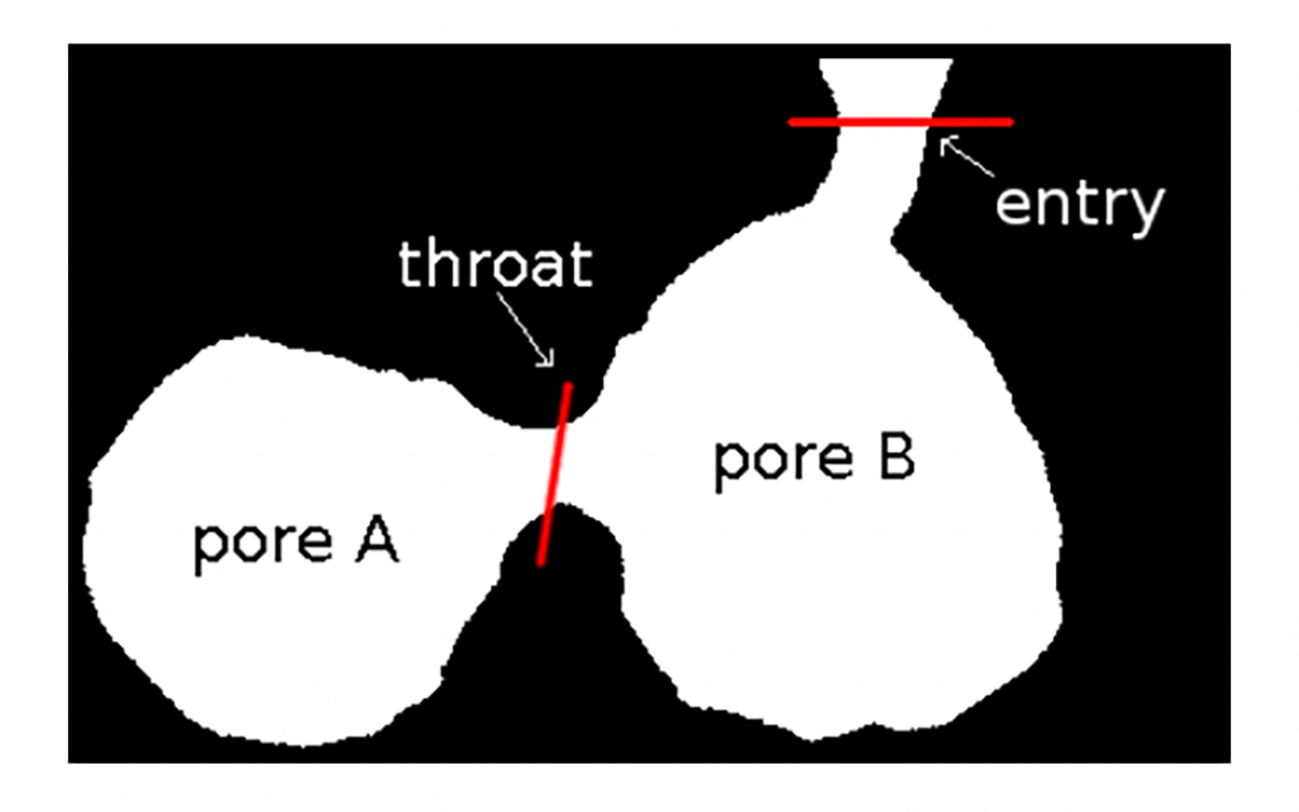
Geometrical and topological representations of the internal structures of samples used in Bio-CAD (bones, biomaterials, rocks and other material samples) are necessary to evaluate their physical properties. Such samples have two disjoint spaces, the pore space and solid space; thus, they can be represented with binary models. The pore space, in turn, is made up of a collection of pores that can be intuitively defined as local openings interconnected by narrow apertures called throats that limit the access to a larger pore (Garboczi, Bentz & Martys, 1999) (Figure 1).
Usually, porous datasets are considered adequate for analysis if they have their holes homogeneously distributed along the sample, and the pore size is notably smaller than the dataset size (Garboczi et al., 1999); that is, they contain complete holes and the object resolution is high enough to clearly define their shape.
The study of porous materials’ properties is of great utility in several disciplines. In medicine, they are used to evaluate the degree of osteoporosis and the adequacy of synthetic biomaterial implants for bone regeneration, among other applications. Bone regeneration occurs in the cavities of the implants where blood can flow. Biomaterial implants can be designed as tissue scaffolds, that is, extracellular matrices onto which cells can attach and then grow and form new tissues (Giannitelli, Accoto, Trombetta & Rainer, 2014; León-Mancilla, Araiza-Téllez, Flores-Flores & Piña-Barba, 2016). In geology, the porous morphology and pore sizes are related to the mineral fabric (Klaver, Desbois, Urai & Littke, 2012) and to its oil-bearing and hydrological properties (Silin, Jin & Patzek, 2004).
Likewise, brine inclusions in sea ice can be formalized in terms of their morphology and pore connectivity (Golden et al., 2007). Silica sands need to have a high sphericity, in that where the rounder and more spherical the particle is, the more resistant that particle is to crushing or fragmenting (Schroth, Istok, Ahearn & Selker, 1996). In engineering, the durability of cementitious materials is associated with certain mechanical and transport properties that can be evaluated based on the properties of the pore space (Stroeven & Guo, 2006).
There are several methods for describing porous materials. Some of them have been traditionally computed using 2D methodologies, and their results extended to 3D by means of stereologic techniques, while other parameters can be computed directly from the volume dataset.
Background
Pore-size distribution
Pore-size distribution is usually computed with mercury intrusion porosimetry (MIP), an in-vitro experiment based on the capillary law governing liquid penetration into small pores. In this technique, mercury is intruded into the sample at increasing pressures, causing the fluid to flow through smaller apertures.
Virtual porosimetry is an in-silico experimentation for general porous materials that simulates MIP at incremental pressures (Garboczi et al., 1999). All separated components of the pore space filled at a given pressure are considered pores and labeled with the diameter corresponding to the applied pressure. This is a flood-fill methodology that uses a previously computed 2D (surface) skeleton as a guide to simulate mercury intrusion from the entry points into the pore space. Moreover, the skeleton is labeled at each point with the corresponding distance (the maximum radius) used to allow or stop the mercury intrusion simulation, i.e., when this radius is smaller than the radius for the current pressure, the simulated intrusion at this pressure stops. Regions corresponding to these smaller radii are the throats. This method is applied to biomaterial samples (Vergés, Ayala, Grau & Tost, 2008b) and soil samples (Delerue, Lomov, Parnas, Verpoest & Wevers, 2003). The latter uses the obtained pore network to compute the permeability. Several methods define the initial set of entry points as those pore voxels which are connected to exterior; however, it can be predefined to allow more freedom to the user in the simulation.
There are other methods that do not require skeleton computation to simulate MIP (Rodríguez, Cruz, Vergés & Ayala, 2011); instead, they use an iterative process that considers the diameters corresponding to pressures. At each iteration, geometric tests detect throats for the corresponding diameter, and a connected-component labeling process collects the region invaded by the mercury.
There are other approaches to compute the pore-size histogram and the pore graph. Some are related to the shape-analysis discipline and use a 2D skeleton as a tool to devise the shape and size of pores. These approaches are heuristic methods that cover the pore space with overlapping spheres, so that the pores are computed as the unions and differences of maximal spheres centered at skeleton points. These methods can be applied to sand samples (Silin et al., 2004), bone scaffolds (Cleynenbreugel, 2005), and biomaterial samples (Vergés et al., 2008a).
Other approaches based on the 1D (curve)-skeleton computation detect throats as the absolute minima of the skeleton. Thus, pores are defined as the regions limited by throats and solid space (Lindquist & Venkatarangan, 1999). A graph is obtained directly from the 1D skeleton, in which nodes correspond to pores and edges to throats (Liang, Ioannidis & Chatzis, 2000). Alternatively, the minimal cost paths connecting boundary points can be computed instead of skeletons to allow methods based on porosimetry, as well as sphere positioning, to be applied (Schena & Favretto, 2007).
Another technique for computing pore-size histograms is granulometry. This methodology consists in the application of successive morphological openings and does not require the computation of a skeleton (Cnudde, Cwirzen, Maddchaele & Jacobs, 2009; Hilpert & Miller, 2001; Schulz, Becker, Wiegmann, Mukherjee & Wang, 2007; Vogel, Tölke, Schulz, Krafczyk & Roth, 2005). A specific set of discrete spheres with diameters D such that S(D) ⊂ S(D+1) can be used, thereby ensuring that a larger ball will never reach a cavity in which a smaller ball cannot enter (Hilpert & Miller, 2001). Physical MIP has been compared with a granulometry-based method (Cnudde et al., 2009).
Throats can also be detected based on the negative Gaussian curvature of the surface. This method is used to decompose the solid space into single particles and to compute mechanical properties such as grain size and coordination number (number of contacts per grain) (Theile & Schneebeli, 2011).
Representation Models
In most of the reported literature, the operations to study binary volume datasets are performed directly on the classical voxel model. However, in the field of volume analysis and visualization, several alternative models have been devised for specific purposes.
Hierarchical structures such as octrees and kd-trees have been used for Boolean operations (Samet, 1990), connected-component labeling (CCL) (Dillencourt, Samet & Tamminen, 1992), and thinning (Quadros, Shimada & Owen, 2004; Wong, Shih & Su, 2006). Octrees are used as a means of compacting regions and getting rid of the large amount of empty space in the extraction of isosurfaces (Wilhems & Gelder, 1992). Their hierarchy is suitable for multi-resolution when dealing with very large data sets (Andújar, Brunet & Ayala, 2002; LaMar, Hamann & Joy, 1999), as well as to simplify isosurfaces (Vanderhyde & Szymczak, 2008). Kd-trees have been used to extract two-manifold isosurfaces (Greß & Klein, 2004).
There are models that store surface voxels, thereby gaining storage and computational efficiency. The semi-boundary representation affords direct access to surface voxels and performs fast visualization and manipulation operations (Grevera, Udupa & Odhner, 2000). Certain methods of erosion, dilation and CCL use this representation (Thurfjell, Bengtsson & Nordin, 1995). The slice-based binary shell representation stores only surface voxels and is used to render binary volumes (Kim, Seo & Shin, 2001).
In this paper, the Compact Union of Disjoint Boxes (CUDB) decomposition model is used. With this model the geometry is partitioned in a non-hierarchical, sweep-based way. An algorithm has been devised to detect the throats based on this model.
OPP and the CUDB model
A binary voxel model represents an object as the union of its foreground voxels, and its continuous analog is an orthogonal pseudo-polyhedra (OPP) (Lachaud & Montanvert, 2000). OPP have been used in 2D to represent the extracted polygons from numerical control data (Park & Choi, 2001). Some 3D applications of OPP are: general computer graphics applications, such as geometric transformations and Boolean operations (Bournez, Maler & Pnueli, 1999; Esperança & Samet, 1998); skeleton computation (instead of iterative peeling techniques) (Eppstein & Mumford, 2010; Martı́nez, Pla & Vigo, 2013); orthogonal hull computation (Biedl & Genç, 2011; Biswas, Bhowmick, Sarkar & Bhattacharya, 2012); boundary extraction (Vigo, Pla, Ayala & Martínez, 2012); and model simplification (Cruz-Matías & Ayala, 2014). OPP have been also used in theory of hybrid systems to model the solutions of reachable states (Bournez et al., 1999; Dang & Maler, 1998).
The Compact Union of Disjoint Boxes (CUDB) (Cruz-Matías & Ayala, 2017) is a special kind of spatial partitioning representation, where an OPP is decomposed in a list of disjoint boxes. These models can be obtained from the voxel model and other alternative models. The conversions algorithms have been published (Cruz-Matías & Ayala, 2017).
Let P be an OPP and Π
c
a plane whose normal is parallel (without loss of generality) to the X
axis, intersecting it at x = c, where
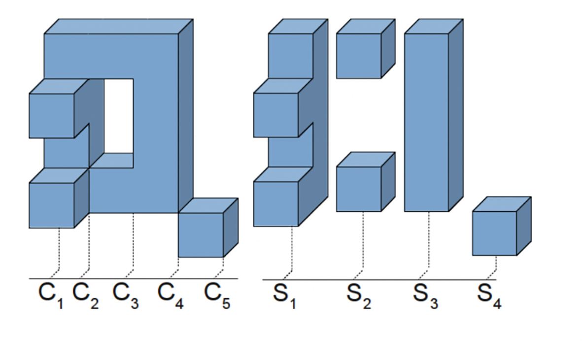
Source: Authors’ own elaboration.
Figure 2 Left: an orthogonal polyhedron with five cuts. Right: its sequence of four prisms with the representative sections (X direction).
An OPP can be represented with a sequence of orthogonal prisms represented by their section. Moreover, if the same reasoning is applied to the representative section of each prism, an OPP can be represented as a sequence of boxes. CUDB represents an OPP with such an ordered sequence of boxes in a compact way, as many boxes generated by the aforementioned split process are merged into one in several parts of the model. CUDB is axis-aligned like octrees and bintrees, but the partition is done along the object geometry as in binary space partitioning (BSP). Depending on the order of the axes, chosen to split the data, a 3D object can be decomposed into six different sets of boxes: XYZ, XZY, YXZ, YZX, ZXY, ZYX, and the set will be ordered according to the chosen configuration. Figure 3 illustrates two possible decompositions of the model in Figure 2 (left). In 2D, an object can be decomposed into two different sets: XY and YX.
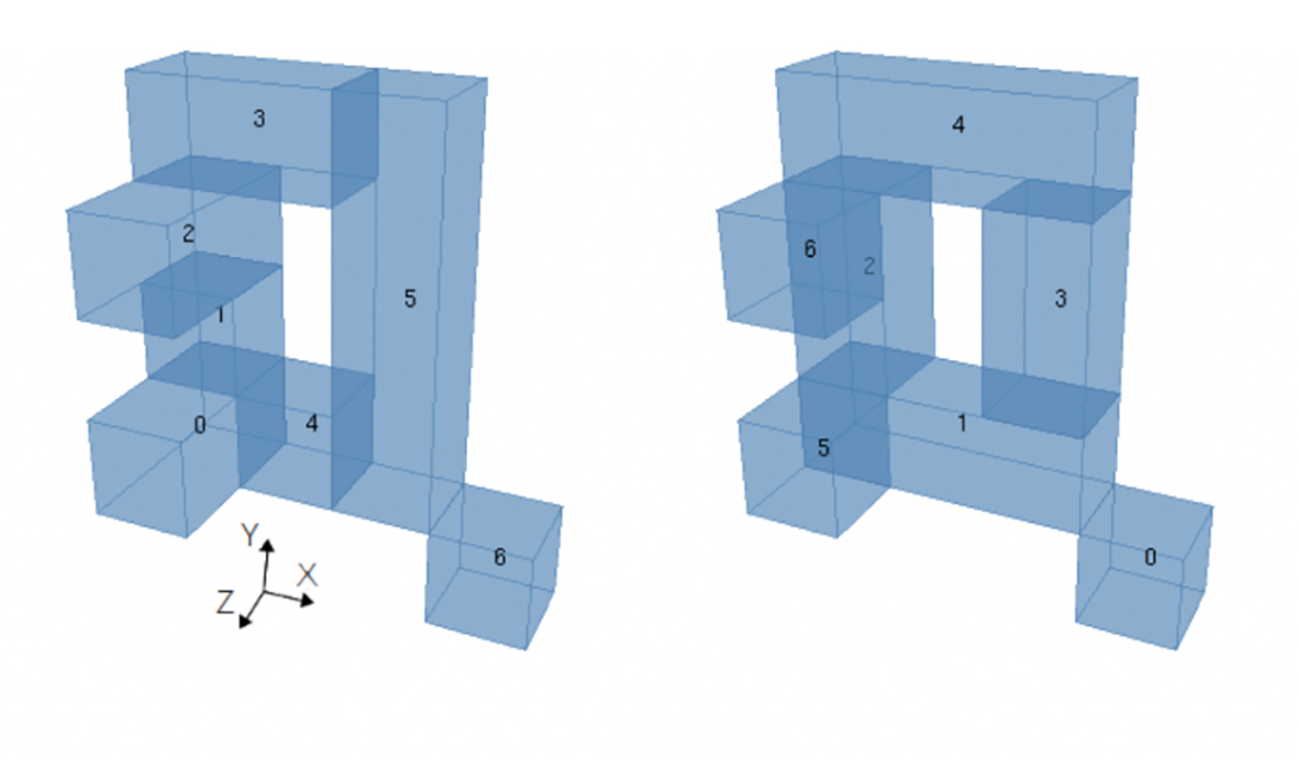
Source: Authors’ own elaboration
Figure 3 XYZ-CUDB (left) and ZYX-CUDB (right) representation for the model in Figure 2, both with seven boxes.
In the CUDB model, the adjacency information of the boxes is stored. Each box has neighboring boxes in only two orthogonal directions: A- and B-direction, and for each one there are two opposite senses; so, four arrays of pointers to the neighboring boxes (two for each direction) are enough to preserve the adjacency information that is required for future operations. These arrays are defined as A-backward neighbors (ABN), A-forward neighbors (AFN), B-backward neighbors (BBN) and B-forward neighbors (BFN). For more details of this model see (Cruz-Matías & Ayala, 2017).
Methodology
Geometric Pore Space Partition
Unlike traditional approaches, which require the skeleton, the method adopted in this study uses the 2D CUDB-encoded pore space as input. It consists of two different sorted sets of boxes for 2D samples, in which a box represents a cluster of pixels.
The basic steps of our algorithm are:
Remove Unreachable Regions
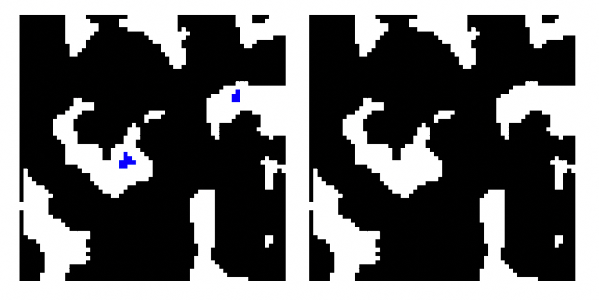
As in real porosimetry, only those components connected to the exterior (reachable components) are able to be filled, so totally interior components (cavities) will not be considered.
In order to remove the unreachable regions, a CUDB-based connected component labeling is applied, where those boxes that are connected to the exterior are labeled with the same label; boxes with a different label are removed. Figure 4 illustrates the removal process with a 2D example.
2D Throats Detection
In the method used in this study, throats can be orthogonal or oblique and all of them are shaped as lines (Figure 5). In order to detect orthogonal and oblique throats, the pore space must be exhaustively scanned in the two 2D main directions.

Orthogonal Throats Detection
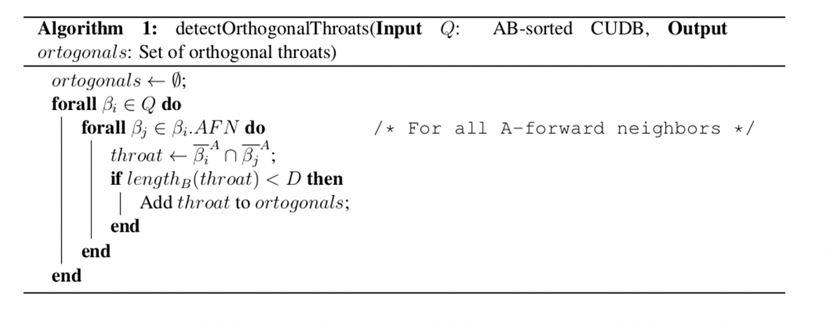
Boxes in 2D-CUDB have neighboring boxes only in the A-direction; therefore, orthogonal throats can exist in any of these directions. As the main axis that splits the model is A, orthogonal throats are detected in this direction. Thus, the two AB-sorted CUDB encodings of the pore space are required to detect all orthogonal throats.
Let β
i
and β
j
be two A-adjacent boxes and
Note that the orthogonal throat is the intersection of two adjacent boxes, as shown in Figure 5 (left) and Figure 5 (middle). Algorithm 1 shows the steps of the orthogonal throat detection process for a single AB-sorting (Figure 6).
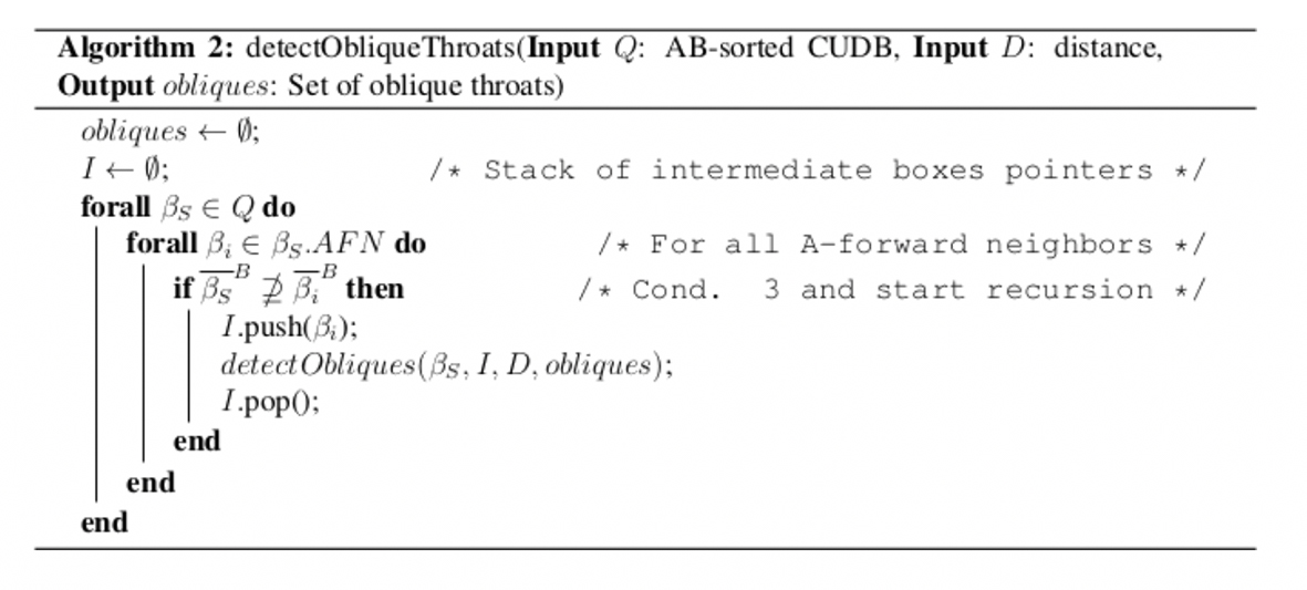
Oblique Throats Detection
Note that an oblique 2D throat is an oblique segment. The next process generates the oblique throats for an AB-sorted CUDB which, due to the characteristics of the CUDB model, are the same generated for the corresponding BA-sorted CUDB.
Let β
i-1
, β
i
and β
i-1
be three consecutive A-adjacent boxes in an AB-sorted CUDB, and let
Source: Authors’ own elaboration.
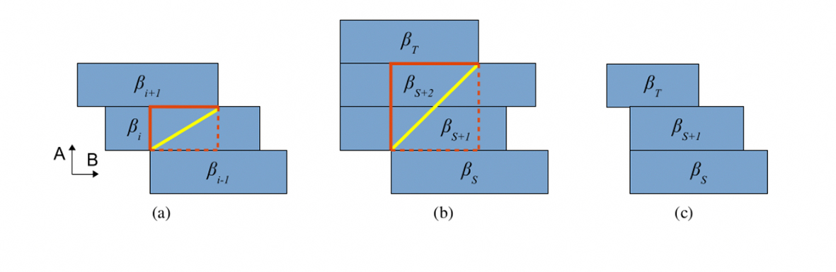
Figure 7 Oblique throats. (a) Simplest case of oblique throat (with just one intermediate box). (b) Oblique throat with more than one intermediate box. (c) Non oblique throat.
However, oblique throats are not restricted to three consecutive boxes. Depending on the geometry of the object, an oblique throat can occur between two boxes, β S and β T , which have more than one intermediate box between them, as shown in Figure 6 (b) . In these cases, all the previous conditions must be satisfied for β S and β T instead of β i-1 and β i+1 , respectively. Therefore, these conditions are rewritten as:
Condition 1 means that
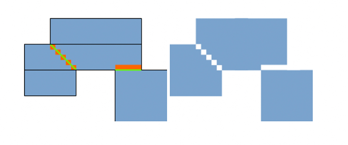
The previous conditions are used to detect an oblique throat between β S and β T . Although a rectangle is obtained (see the rectangle highlighted in orange color in Figures 7a and 7b), the strategy to compute the throat is by considering the diagonal included in the mentioned rectangle (see the inclined line highlighted in yellow color in Figures 7a and 7b). This strategy allows to separate the pore space in two regions in the current scan direction.
A box β S can generate several oblique throats with its consecutive boxes in the A-direction (Figure 8a). Therefore, in order to detect all the possible oblique throats, all consecutive boxes of β S must be scanned. The method used here searches for any configuration that satisfies the oblique throat conditions.
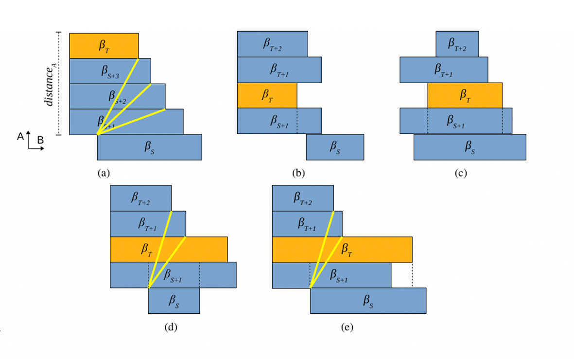
Source: Authors’ own elaboration.
Figure 8 2D oblique throats scanning process. (a) A box that generates several oblique throats. (b) Condition 1 is not satisfied. (c) Condition 3 is not satisfied. (d) Condition 2 is not satisfied. (e) Condition 4 is not satisfied.
Conditions 1 and 3 are required conditions to stop the search process, while the others are not. The search stops in case that Condition 1 is not satisfied, as every subsequent box β T will not satisfy Condition 4 in the following iterations (Figure 7). When Condition 1 is not satisfied, every subsequent box β T will not either satisfy Condition 2 or 4 in the following iterations (Figure 7). Moreover, the search must be also stopped when the distance between β S .V1 and β T .V1 in the A-coordinate is greater than a certain distance D, this distance has been defined as the smaller dimension of the model. However, when conditions 2 and 4 are not satisfied, there may still be subsequent boxes that define throats that satisfy all conditions (Figures 8d and 8e).
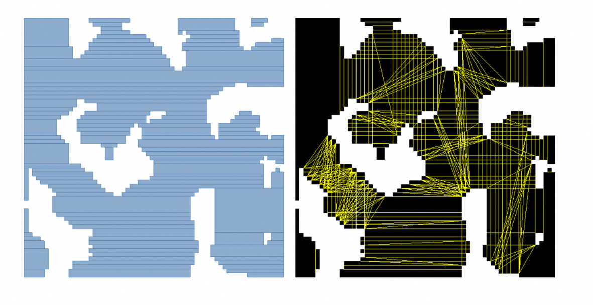
Algorithms 2 and 3 show the steps of the oblique throat detection using a recursive strategy for a single AB-sorting (Figure 9 and 10). Figure 11 shows an example of throats computation. In this Figure, black and white represent the pore and solid spaces respectively.

Partitioning of the Pore Space
An accurate identification of pore throats is important in the partitioning of the pore space. It is necessary to be careful not to generate too many throats which can produce a large number of small pores, which would correspond primarily to the roughness of the pore wall interface.
From the point of view of the utility of the resulting pore and throats size distributions in network simulations, it is desirable to partition the pore space into nodal pores (pores that are also topological nodes) separated by throat cross-sectional surfaces (Ioannidis, Chatzis & Kwiecien, 1999). This is possible if pore necks are identified as the minimum distance that connect the solid space. In methods like those by Liang et al. (2000) and Lindquist & Venkatarangan (1999), throats are identified through a search for minima in the hydraulic radius of individual pore space, where each branch of the skeleton (link) is considered as a separate pore.
Although the method used follows the previous idea, the authors of the study do not rely on prior computation of the skeleton; instead, all the possible throats generated with the strategy described below are computed, then, such throats are analyzed in order to obtain those that better split the pore space.
The strategy to split the pore space is to determine the shortest throats that join the solid regions. Therefore, the first step consists in sorting the detected throats by length. To obtain the solid regions, a CCL process is applied to the CUDB-encoded solid space. For instance, Figure 11 shows that this sample has 10 solid regions.
Once the throats have been sorted and the solid regions have been detected, it is necessary to determine the final throats that will split the pore space. Let S A and S B be two solid regions, each of the ordered throats is analyzed to obtain the pair (S A , S B ) joined by this throat. This detection is done by evaluating each box of each CUDB-encoded solid region. However, this process can be speeded up by using the bounding box to do previous discards.
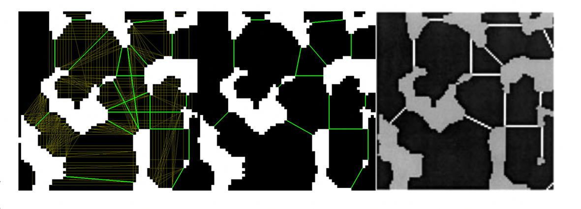
Figure 12 (left) shows the resulting throats after the previous strategy. Note in this sample that although there are no throats joining the same solid regions, several intersected throats exist. Some of these throats are longer than some paths formed by other throats. This problem can be solved by applying a Dijkstra's algorithm (Dijkstra, 1959). Every time a throat is found for the pair (S A , S B ), it is examined whether there is a shorter path formed with previously calculated throats; if this is the case, the throat is omitted. Implementation of these criteria is shown in Figure 12 (middle).
Source: Authors’ own elaboration.
Figure 12 Partitioning of the pore space. Left: partitioning at the resulting throats (21 throats). Middle: Implementation of the final criteria to detect throats (15 throats). Right: Partitioning using a skeleton-based method.
Once the final throats have been detected, the object is subdivided along each one of them to partition the pore space into its constituent pores. To achieve this subdivision, a unit-width orthogonal polygon 2D is built for each throat. This OPP is obtained by the 2D scan-conversion of the segment which represent the throat. Therefore, the difference between the OPP-object and the OPP-throat produces the object subdivided along the throat. Figure 13 illustrates the subdivision of the object along two oblique throats.
Source: Authors’ own elaboration.
Figure 13 Left: Scan conversion of one orthogonal and one oblique throat. Right: Difference between the object and the scan-converted segments.
Once the pores have been correctly separated, their area is straightforward computed using the CUDB-encoded pore.
Results and discussion
The method presented here, like those based on prior computation of the skeleton, is a geometric approach that computes the expected solution.
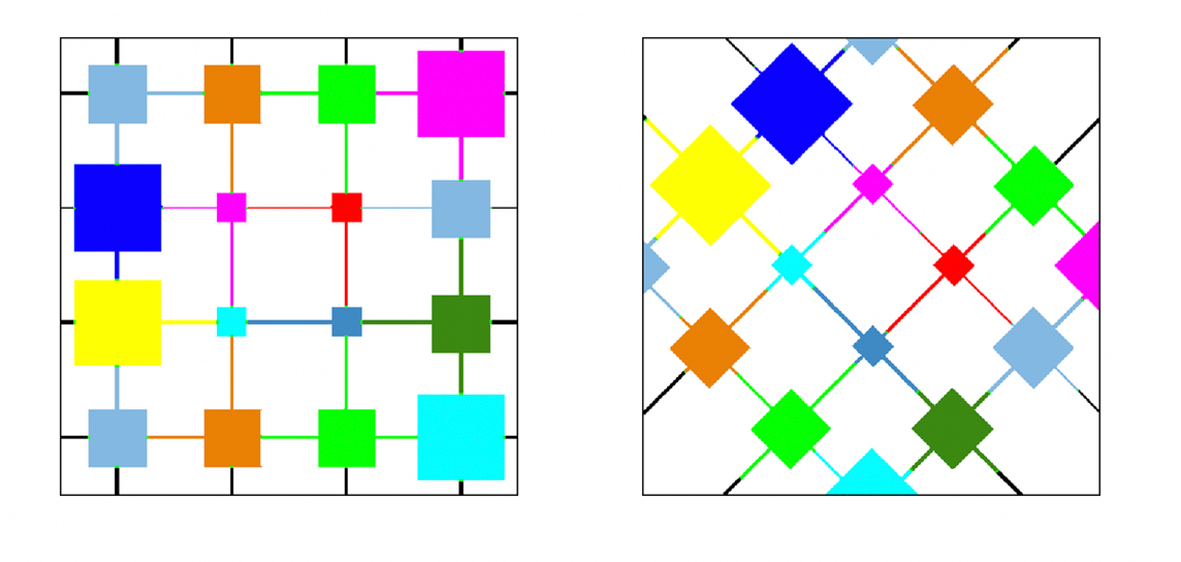
Figure 14 shows a well-defined structure for which it is easy to determine the theoretical solution. This model has a size of 450 x 450 pixels and contains squares of 85, 58 and 30 pixels per side connected with small lines (throats) of size 2 and 4 pixels. Note in this figure that the method is invariant to rotation to detect the throats and to divide the pore space correctly. For more clarity, the pores after the subdivision along the throats have been colored.
Source: Authors’ own elaboration.
Figure 14 Model of squares. Left: Original 450 × 450. Right: Model rotated 45 clockwise.
The adopted approach has been compared with a skeleton-based approach. The model used to explain the partitioning process is the same used in Liang et al. (2000). In Figure 9 (middle and right) both methods get a quite similar partitioning of the pore space.
Also, the effects of resolution on the method used here have been tested. Resizing the image does not affect the topology of the detected throats. Although the bigger the image, the more throats are generated, the method to detect the final throats allows to obtain an almost identical pore space partition. Figure 15 shows the minor effects with increasing resolution. Of course, the accuracy of measurements is expected to increase as resolution increases.
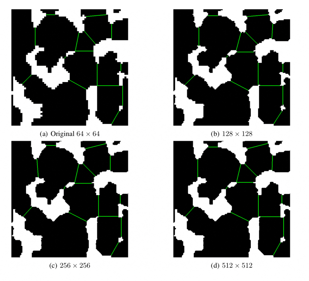
Source: Authors’ own elaboration.
Figure 15 Effects of increasing the size of the image in the method used in this research.
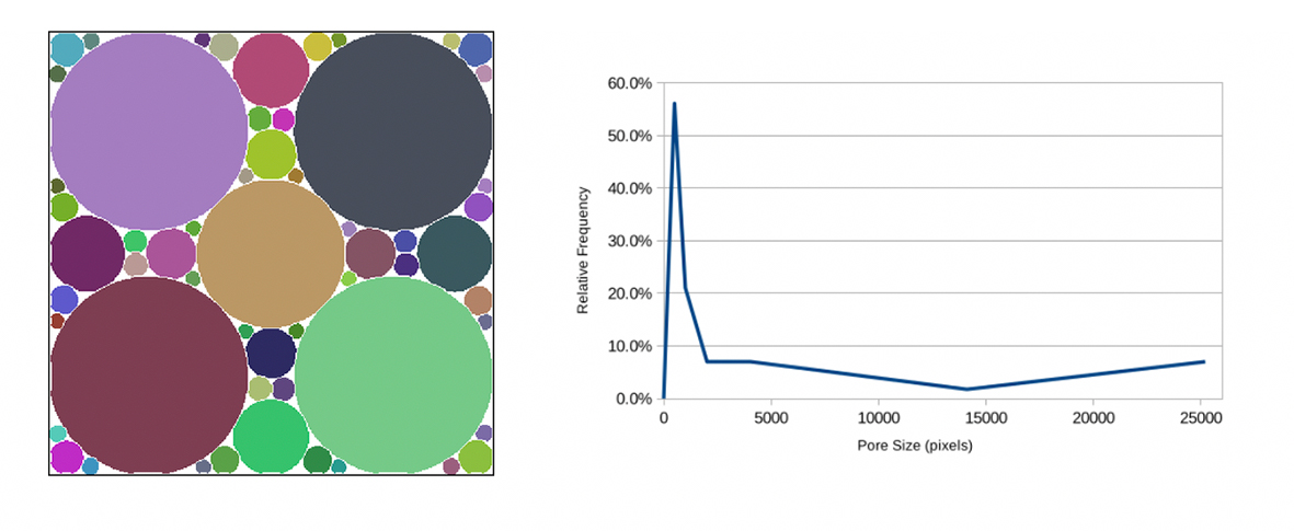
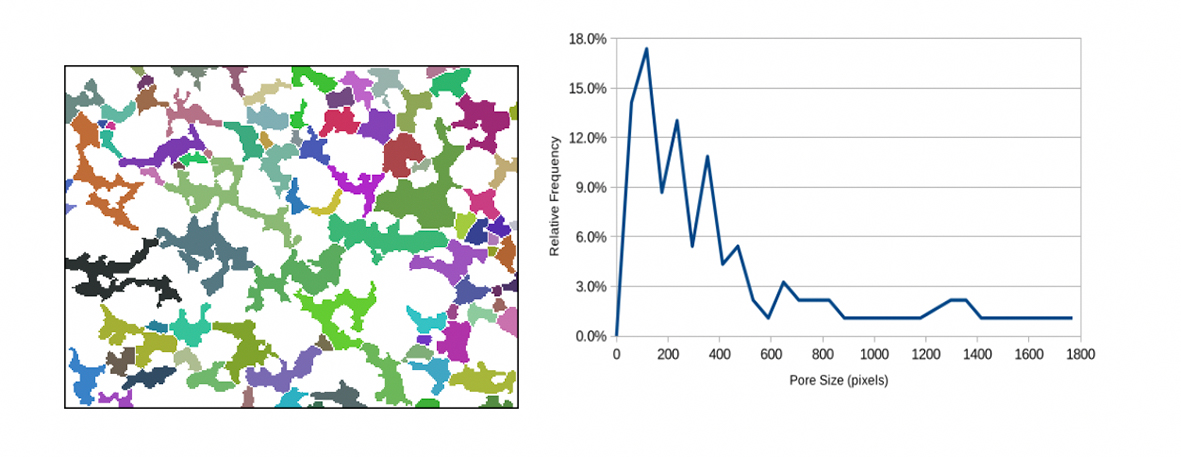
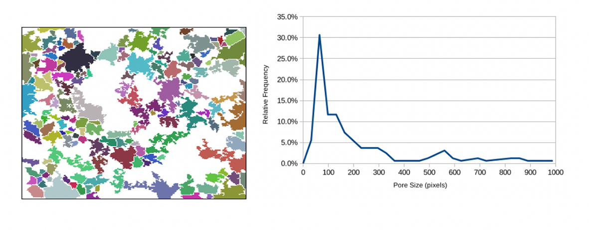
Finally, sections of several real porous samples have been tested, as shown and described in Table 1 below. Figures 16 to 19 depict the corresponding partitioned porous space and its pore-size distribution.
Spheres: A synthetic model with spheres of a variable size.
PLA: A biomaterial sample consisting of polylactic acid (PLA) with a 16 µm3 voxel resolution.
Soygel: Sample of hydroxyapatite with a soy-based foaming agent for bone prosthetics with a 16 µm3 voxel resolution.
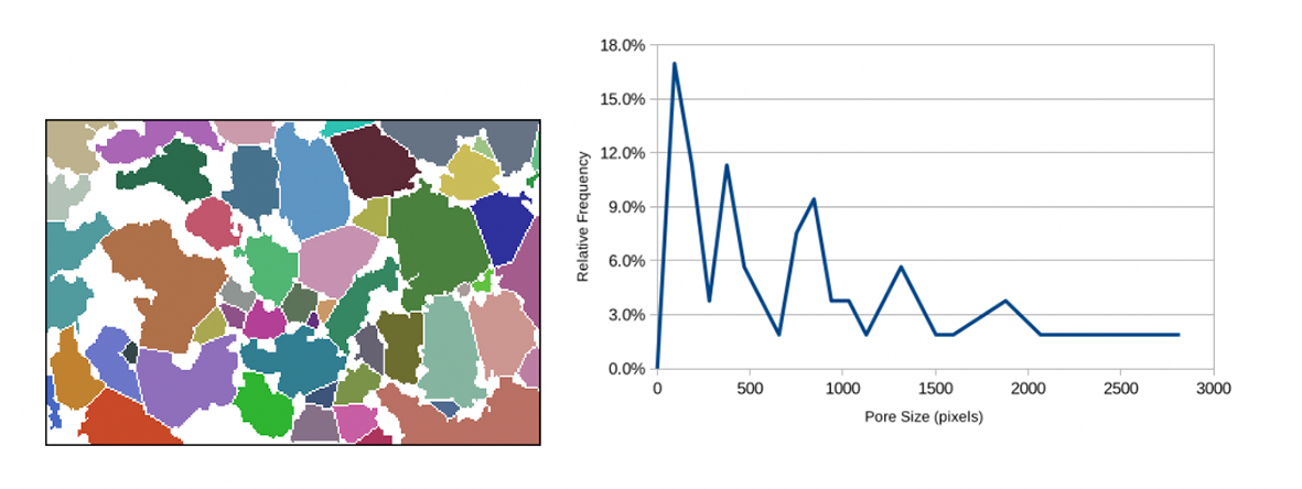
Stone: A stone sample consisting of sedimentary rock from a Lybian oil-bearing unit with a 4.4 µm3 voxel resolution.
Table 1 Datasets. For each dataset: size of the sample in pixels, run time (in milliseconds) to partition the pore space.
| Dataset | Size | Time (ms) |
| Spheres | 450 x 540 | 96 |
| PLA | 314 x 237 | 56 |
| Soygel | 251 x 251 | 843 |
| Stone | 271 x 179 | 25 |
Source: Authors’ own elaboration.
Source: Author’s own elaboration.
Figure 16 Spheres: A synthetic model. Left: Partitioned porous space. Right: Pore-size distribution.
Source: Author’s own elaboration.
Figure 17 PLA: A biomaterial sample. Left: Partitioned porous space. Right: Pore-size distribution.
Source: Author’s own elaboration.
Figure 18 Soygel: Sample of hydroxyapatite. Left: Partitioned porous space. Right: Pore-size distribution.
Source: Author’s own elaboration.
Figure 19 Stone: A stone sample. Left: Partitioned porous space. Right: Pore-size distribution.
All the real samples have been scanned by Trabeculae® and segmented by thresholding and applying noise filtering. The corresponding programs have been written in C++ and tested on a PC Intel®Core i7-4600M CPU@2.90GHz with 7.6 GB RAM and running Linux.
Based on the analysis of the figures and the histograms, it can be concluded that the obtained pore size distribution is accurate enough. A more detailed discussion of the comparison of physical and in-silico experimentation is beyond the scope of this paper.
Conclusions
A new method to characterize the pore space has been proposed; it does not require prior computation of the skeleton. As this prior preprocessing is very time-consuming, this approach achieves a noticeable reduction in time. The key feature of the presented method is the process to determine the throats that make it possible to separate regions corresponding to different pores.
The in-silico approaches are based on the geometry of the analyzed samples, and the results obtained are the expected theoretical results, as shown in the results section.
As a future work, several topics must still be studied. At present, the authors are starting to study how to extend this method directly to 3D models and will make contact with biomaterials and geology research teams that provide new problems to study and other kinds of real samples. Further, new methods will be developed for other parameters, such as connectivity and anisotropy. Moreover, the authors of this research are also interested in applying time-varying techniques based on a CUDB model.

