


 nova página do texto(beta)
 Inglês (pdf)
 Artigo em XML
 Referências do artigo
 Enviar este artigo por email
 Citado por SciELO
  Similares em
SciELO
Similares em
SciELO 
 Permalink
Introducción
Troesch’s equation is important in physics because it models the confinement of a plasma column by radiation pressure. Thus, it is relevant to search for precise solutions for this equation. Unfortunately, Troesch’s equation is difficult to solve, as it happens with several nonlinear differential equations that appear in the physical sciences.
Laplace transform (LT) has played a relevant role, not only for its theoretical interest but also for its methods that allow to solve, in a simpler way, ordinary differential equations (ODE) that model many problems in the fields of engineering and science, in comparison with other mathematical methods (Spiegel, 1988). Specifically, LT has been useful for the solution of ODE with constant coefficients and initial conditions; also, LT can be employed in the case of certain differential equations with variable coefficients and partial differential equations (Spiegel, 1988). The applications of LT for nonlinear ODES has been focused, mainly, on getting analytical approximate solutions. Thus, Aminikhah & Hemmatnezhad (2012) reported LT-HPM, which is a coupling of the homotopy perturbation method (HPM) and LT methods aiming to get precise approximate solutions for these equations. Nevertheless, just as it happens with LT, LT-HPM has been employed, above all, to solve problems with initial conditions (Aminikhah, 2012a; Aminikhah & Hemmatnezhad, 2012), because LT-HPM is directly related to these problems. This work presents LT-HPM with the goal of finding an approximate solution for the nonlinear ODE that describes Troesch’s problem, which is defined on a finite interval with Dirichlet boundary conditions.
ODE with boundary conditions on infinite intervals has been regarded in some papers, and it often corresponds to problems defined on semi-infinite ranges (Aminikhah, 2012b; Khan, Gondal, Hussain & Vanani, 2011); nevertheless, the way to solve these problems is different from the method presented in this work. The importance of research on nonlinear ODE is that many phenomena, theoretical and practical, have a nonlinear nature. Recently, various methods, alternative to classical methods, have risen to search approximate solutions for nonlinear differential equations, such as variational approaches (Assas, 2007; He, 2007; Kazemnia, Zahedi, Vaezi & Tolou, 2008; Noorzad, Poor & Omidvar, 2008), tanh method (Evans & Raslan, 2005), exp-function (Mahmoudi, Tolou, Khatami, Barari & Ganji, 2008; Xu, 2007), Adomian’s decomposition method (ADM) (Adomian, 1988; Babolian & Biazar, 2002; Chowdhury, 2011; Deeba, Khuri & Xie, 2000; Kooch & Abadyan, 2011; 2012; Vanani, Heidari & Avaji, 2011), parameter expansion (Zhang & Xu, 2007), homotopy perturbation method (HPM) (Aminikhah, 2012a; 2012b; Aminikhah & Hemmatnezhad, 2012; Araghi & Rezapour, 2011; Araghi & Sotoodeh, 2012; Bayat, Bayat & Pakar, 2014; Bayat, Pakar & Emadi, 2013; Belendez et al., 2009; Biazar & Aminikhah, 2009; Biazar & Eslami, 2012; Biazar & Ghanbari, 2012; Biazar & Ghazvini, 2009; El-Shaed, 2005; Feng, Mei & He, 2007; Fereidon, Rostamiyan, Akbarzade & Ganji, 2010; Filobello-Niño et al., 2012a; 2012b; 2015; Ganji, Mirgolbabaei, Miansari & Miansari, 2008; He, 1999; 2000; 2006a; 2006b; Khan et al., 2011; Khan & Wu, 2011; Marinca & Herisanu, 2011; Mirmoradia, Hosseinpoura, Ghanbarpour & Barari, 2009; Madani, Fathizadeh, Khan & Yildirim, 2011; Rashidi, Pour, Hayat & Obaidat, 2012; Rashidi, Rastegari, Asadi & Beg, 2012; Sharma & Methi, 2011; Vazquez-Leal et al., 2012; Vazquez-Leal et al., 2013; Vazquez-Leal et al., 2014; Vazquez-Leal, Castañeda-Sheissa, Filobello-Niño, Sarmiento-Reyes & Sanchez-Orea, 2012; Vazquez-Leal, Filobello-Niño, Castañeda-Sheissa, Hernandez-Martinez & Sarmiento-Reyes, 2012; Vazquez-Leal, Sarmiento-Reyes, Khan, Filobello-Nino & Diaz-Sanchez, 2012), homotopy analysis method (HAM) (Hassana & El-Tawil, 2011; Patel, Mehta & Pradhan, 2012), and perturbation method (PM) (Filobello-Niño et al., 2013a), among others. In the same way, some exact solutions to nonlinear ODE have been introduced, for example, in Filobello-Niño et al. (2013b).
The organization of this work is as follows. Section Standard HPM introduces the basic idea of the Homotopy Perturbation Method. The next Section presents the LT-HPM method. In Case Study section, LT-HPM is presented in order to find an approximate solution for Troesch’s equation. Additionally, a discussion on the results is presented. Finally, a conclusions section presents the results obtained from this work.
Standard HPM
The HPM method was introduced with the aim to find approximate solutions to various kinds of nonlinear problems. Indeed, HPM is a combination of the classical perturbative technique and the homotopy, whose origin is found in the topology, but it is not restricted to small parameters. Besides, HPM often requires a few iterations to find accurate approximate solutions (He, 2000; 1999).
To understand how the HPM method works, consider a general nonlinear differential equation (He, 2000) expressed as:
with boundary conditions
Where A is a differential operator, B is a
boundary operator, f (r) is a known analytical function and
where L is linear and N nonlinear.
In general, a homotopy is constructed as follows (He, 1999; 2000):
or
Where p is called the homotopy parameter, while u 0 is the first approximation for the solution of (3) that satisfies the boundary conditions.
The solution for (4) or (5) is expressed as:
By substituting (6) into (5) and comparing identical powers
of p terms, there can be found values for
After considering p→1, the following approximate solution for (1) is obtained:
Basic Idea of Laplace Transform Homotopy Perturbation Method (LT-HPM)
The aim of this section is to show how LT-HPM is used with the purpose of obtaining approximate solutions for ODE, as (3) (Aminikhah, 2012b; Filobello-Nino et al., 2015).
The procedure for LT-HPM follows the same steps as HPM, but only until (5); next, LT is applied on both sides of (5) to get:
From Spiegel (1988), the following is obtained:
or
Applying inverse Laplace transform to both sides of (10), the following is obtained:
Next, it is assumed that the solutions of (3) are expressed as:
so that substituting (12) into (11) be:
After comparing coefficients with the same power of p :
Assuming that the initial approximation adopts the form
Case Study
Next, LT-HPM is used in order to get a handy analytical approximate solution for the nonlinear problem:
where
The terms to be identified are
and
where prime denotes differentiation respect to x.
Next, on the right side of (16), in terms of its Taylor series, the following is expressed:
In order to show the usefulness of the proposed method, an accurate approximate solution will be obtained, keeping only the first two terms on the right side of (19).
Next, the following homotopy is constructed (see 4):
or
After applying LT:
Following Spiegel (1988), the (22) is rewritten as:
where
After using
Where
Solving for
Next, the following series solution for
It is noted that
is the first approximation for the solution for (16), which satisfies the conditions
Thus, after substituting (26) into (25), the following is obtained:
After comparing coefficients of identical powers of
After solving Laplace transforms (29), (30), and (31):
and so on.
By substituting (32)-(34) into (15), and considering the limit
value
In order to calculate the value of
and
are obtained, respectively.
By substituting (36), (37), and (38) into (35), the following expressions are obtained:
Discussion
This article employed LT-HPM in the search for a handy and precise analytical
approximate solution for the nonlinear ODE defined with finite boundary conditions
that describe the Troesch’s problem. Since the proposed method is expressed in terms
of initial conditions for a given problem (see (14), this procedure consisted of expressing the approximated
solutions in terms of
Figure 1 shows the comparison between numerical
and approximate solutions (39)-(41) for the cases
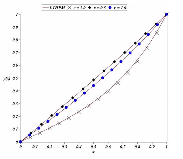
Source: Authors’ own elaboration.
Figure 1 Comparison of proposed solution (35) (solid lines) for,
Table 1 shows the comparison between the
exact solution reported by Erdogan & Ozis
(2011), and approximations (39), ADM (Deeba et
al., 2000), HPM (Feng et
al., 2007), HPM (Mirmoradia
et al., 2009), and HAM (Hassana & El-Tawil, 2011) for the case
Table 1 Comparison between (39), the exact solution (Erdogan & Ozis, 2011), and other reported approximate
solutions using
| x | Exact (Erdogan & Ozis, 2011) | This work, LT-HPM (39) | ADM (Deeba et al., 2000) | HPM (Feng et al., 2007) | HPM (Mirmoradia et al., 2009) | HAM (Hassana & El-Tawil, 2011) |
|---|---|---|---|---|---|---|
| 0.1 | 0.0959443493 | 0.09594500637 | 0.0959383534 | 0.0959395656 | 0.095948026 | 0.0959446190 |
| 0.2 | 0.1921287477 | 0.1921300635 | 0.1921180592 | 0.1921193244 | 0.192135797 | 0.1921292845 |
| 0.3 | 0.2887944009 | 0.2887963775 | 0.2887803297 | 0.2887806940 | 0.288804238 | 0.2887952148 |
| 0.4 | 0.3861848464 | 0.3861874818 | 0.3861687095 | 0.3861675428 | 0.386196642 | 0.3861859313 |
| 0.5 | 0.4845471647 | 0.4845504381 | 0.4845302901 | 0.4845274183 | 0.4845599 | 0.4845485110 |
| 0.6 | 0.5841332484 | 0.5841370824 | 0.5841169798 | 0.5841127822 | 0.584145785 | 0.5841348222 |
| 0.7 | 0.6852011483 | 0.6852053362 | 0.6851868451 | 0.6851822495 | 0.685212297 | 0.6852028604 |
| 0.8 | 0.7880165227 | 0.7880205903 | 0.7880055691 | 0.7880018367 | 0.788025104 | 0.7880181729 |
| 0.9 | 0.8928542161 | 0.89285571853 | 0.8928480234 | 0.8928462193 | 0.892859085 | 0.8928553997 |
| AARE | 4.6x10⁻⁶ | 3.47802x10⁻⁵ | 3.57932x10⁻⁵ | 2.44418x10⁻⁵ | 2.51374x10⁻⁶ | |
Source: Authors’ own elaboration.
Table 2 Comparison between (40), the exact solution (Erdogan & Ozis, 2011), and other reported approximate
solutions, using
| x | Exact (Erdogan & Ozis, 2011) | This work, LT-HPM (40) | ADM (Deeba et al., 2000) | HPM (Feng, et al., 2007) | HPM (Mirmoradia,et al., 2009) | HAM (Hassana & El-Tawil, 2011) |
|---|---|---|---|---|---|---|
| 0.1 | 0.0846612565 | 0.08470412291 | 0.084248760 | 0.0843817004 | 0.084934415 | 0.0846732692 |
| 0.2 | 0.1701713582 | 0.1702575190 | 0.169430700 | 0.1696207644 | 0.170697546 | 0.1701954538 |
| 0.3 | 0.2573939080 | 0.2575241867 | 0.256414500 | 0.2565929224 | 0.258133224 | 0.2574302342 |
| 0.4 | 0.3472228551 | 0.3473982447 | 0.346085720 | 0.3462107378 | 0.348116627 | 0.3472715981 |
| 0.5 | 0.4405998351 | 0.4408206731 | 0.439401985 | 0.4394422743 | 0.44157274 | 0.4406610140 |
| 0.6 | 0.5385343980 | 0.5387980978 | 0.537365700 | 0.5373300622 | 0.539498234 | 0.5386072529 |
| 0.7 | 0.6421286091 | 0.6424243421 | 0.641083800 | 0.6410104651 | 0.642987984 | 0.7526899495 |
| 0.8 | 0.7526080939 | 0.7529055047 | 0.751788000 | 0.7517335467 | 0.753267551 | 0.7526899495 |
| 0.9 | 0.8713625196 | 0.8715893682 | 0.870908700 | 0.8708835371 | 0.871733059 | 0.8714249118 |
| AARE | 4.5x10⁻⁴ | 0.002714577 | 0.002320107 | 0.002044737 | 0.0019244326 | |
Source: Authors’ own elaboration.
An important feature from the proposed method is deduced from equations like (16), which are expressed in the
following form
Finally, it is very important to emphasize that it is possible to improve the accuracy of the obtained approximations, adding higher order approximations to the solution (35) and keeping more terms in the Taylor series expansion (19).
Conclusions
In this article, LT-HPM was used to find a polynomial analytical approximate solution of five terms for the second order nonlinear ODE that describes Troesch’s problem with Dirichlet boundary conditions defined on a finite interval. In general, the proposed method expresses the problem of obtaining an approximate solution for a nonlinear ordinary differential equation, in terms of solving an algebraic equation for some unknown initial condition. From Figure 1, and Table 1 and Table 2, it is concluded that LT-HPM is a method with potential in the search for solutions for boundary value nonlinear problems. As it was already mentioned, an additional advantage of LT-HPM is that it does not require to solve several recurrence differential equations; therefore, it can be said that LT-HPM is a useful tool for practical applications.

