


 nueva página del texto (beta)
 Inglés (pdf)
 Artículo en XML
 Referencias del artículo
 Enviar artículo por email
 Citado por SciELO
  Similares en
SciELO
Similares en
SciELO 
 Permalink
INTRODUCTION
Water is essential for all living organisms; it constitutes an indispensable factor for the development of biological processes and natural ecosystems, specifically with respect to the maintenance and reproduction of life on the planet. Different anthropic activities have affected the hydrological cycle (Das and Acharya 2003), thus generating negative consequences for ecosystems, ecosystem biodiversity, and the quality of life for certain populations.
The uncontrolled growth of population, industry, and agriculture creates greater demands for water every day (Ramakrishnaiah et al. 2009). The deterioration in the quality of surface water and groundwater has increased due to population growth, owing to a significant increase in the generation of domestic, industrial, and agricultural wastewater, which contributes to organic, inorganic, and biological contaminants (CONAGUA 2022, SEMARNAT 2020) that are discharged, without treatment, into surface water bodies. As a result of this contamination, many ecosystems show obvious signs of degradation, which in some cases are irreversible; this is in addition to the problems currently being caused by climate change. According to CONAGUA (2022) and SEMARNAT (2020), 70% of the lakes, lagoons, rivers, and other water bodies in Mexico present some degree of contamination and deterioration due to the poor planning of land use in hydrographic basins.
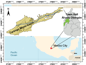
The present case study concerned the Tarango micro-basin, located in southwestern Mexico City and within the Alvaro Obregon District, which includes streams, ravines, and a dam.
The micro-basin covers 378 hectares and has approximately 60 000 inhabitants where the two streams meet, i.e., the Río Puerta Grande and the Río Puente Colorado streams.
In 2009, the Tarango micro-basin was established as an environmental value area (EVA) and was intended solely for conservation and ecological restoration activities. The population releases wastewater into the stream, so there is a risk of contaminating a significant stream reach and lowering its quality, thus affecting the downstream areas and placing the EVA at risk. Despite the deterioration and contamination, the Tarango ravine and the Río Puerta Grande stream still retain much of their environmental potential and represent an essential resource for the region, which is why it is necessary to promote actions that mitigate its damage and restore its quality (PAOT 2010). The region receives approximately 1000 mm of rainwater annually, which means that it could capture a volume of up to 1 235 759.56 m³ of water, which could be used to recharge the Tarango basin (SEMARNAT 2009). In addition, the urbanized hillside of the Tarango ravine represents another 300 hectares that provide as much water, but of the residual type. The problem is that, in the dry season, the predominant type of water is from municipal wastewater discharge, which puts its quality at risk. For the spatial modeling of the Río Puerta Grande stream in Mexico City and for the water quality evaluation, the following physical and chemical parameters were determined: temperature (T ºC), hydrogen potential (pH), total suspended solids (TSS), conductivity (Cond), alkalinity (Alk), hardness (Hard), dissolved oxygen (DO), biochemical oxygen demand (BOD5), nitrates (N-NO3-), phosphates (P-PO43-), and fecal coliform (FC).
ArcGIS software was one of the tools employed to study the spatial distribution of the surface water parameters; the software contains tools such as the IDW interpolator and ArcMap for creating maps (Mtetwa et al. 2003, Najera et al. 2013). Additional software that was used was the GIS tool, which can interpolate with the IDW application and can also build maps with the ArcMap program. IDW is the interpolator that was used to estimate (So) at monitoring site locations. Therefore, “n” is the number of monitoring sites, given the Z(Si) values observed at the sampled locations, as shown in Equation 1 (Ogbozige et al. 2018):
where:
λi |
is the weight of the neighbor i (the sum of the weights could be close to unity to ensure the interpolation) |
Z(Si) |
is the measured value at location i |
So |
is the location of the prediction |
n |
is the number of measured values |
The application of parameter distribution is useful for the evaluation, management, and operation of water resources. Spatial distribution maps play a very important role in the water quality assessment of these water bodies.
A water quality assessment must consider the representative indicators that guarantee the quality of the water resource, which thus allows one to consider what actions are applicable for water management and control. Water quality indices (WQIs) are one of the most widely used multidimensional tools (Coletti et al. 2010). The use of WQIs is increasing as it helps to identify changes in quality, specific environmental conditions, decision making in public policies, and the evaluation of pollution control programs (Ott 1978, Canter 1998, Zhang et al. 2022). In addition, WQIs also support environmental impact studies, such as the identification of water quality in areas with environmental problems (Espinal et al. 2013, Rubio et al. 2014, García et al. 2021). Water quality parameters, whether the water is from a surface river, stream, lake, or groundwater, are important for determining the degree of purity or contamination within a given body of water; furthermore, contaminants can be of physical, chemical, or biological origin. WQIs consider the capacity of the water body to restore its natural properties or the conditions it may have had prior to contamination. One way to know or evaluate the conditions of a water body is to calculate an index that mathematically combines all the water quality measures, and which indicates a generally and easily understood description of its environmental situation. According to Fernández et al. (2004), more than 30 commonly used water quality indices are known, which consider a large range in the number of variables (between 3 and 72). Most of these indices include at least three of the following parameters: dissolved oxygen (DO), biochemical oxygen demand (BOD), ammoniacal nitrogen (N-NH4+), nitrogen in the form of nitrate (N-NO3-), phosphorus in the form of orthophosphates (P-PO43-), potential hydrogen (pH), and total suspended solids (TSS). Horton (1965) was one of the pioneers attempting to generate a unified methodology for calculating a water quality index (WQI). Later, with more significant effort, the U.S.-based National Sanitation Foundation (Kumar and Alappat 2009) conducted a study to evaluate a WQI based on nine parameters. Prati et al. (1971) presented a study with thirteen parameters and Dinius (1972) carried out a similar study with eleven parameters. Among the most widely used WQIs, the one proposed by Brown et al. (1970) stands out, which is a modified version of the water quality index (WQI) developed by the NSF and sees wide dissemination and application. According to Cude (2001), the reviews of water quality indices have been a continuous concern because of their importance, as is evidenced by different studies. As such, new approaches have been generated and these, in turn, have provided new tools for the development of other indices (Dinius 1987, Kung et al. 1992, Dojlido et al. 1994). Among the first comparisons, those of Landwehr and Deininger (1976) stand out, followed by Ott (1978), who carried out a review of the indices used in the United States and provided a detailed discussion on the theory and practice of environmental indices in Europe. In Mexico, Montoya et al. (1997) and León (1991) developed WQIs called ICAS, which were applied by the Mexican National Water Commission (CONAGUA 2017).
According to Torres et al. (2009), WQIs for surface sources are used for water control, mainly for human consumption. Applying a water quality index has the following advantages:
Gives a simple, concise, and valid method that expresses the importance of the data generated in the laboratory.
Identifies water quality trends and defines problem areas.
Prioritizes water quality in detail.
However, its application has limitations since not all the risks present in a body of water can be evaluated due to the cases where there is a presence of toxic substances, which depend on the conditions within the water bodies of a region. There are also cases where the water contains strong contamination and the WQI is close to or equal to 0% (clean waters with excellent conditions are close to 100%).
The objective of this work was to map the variable distribution of 10 water quality parameters for the Tarango micro-basin during the dry season and after the rainy season. ArcGIS, IDW, and ArcMap software were used to analyze data that were recorded at seven monitoring sites.
MATERIALS AND METHODS
Study area and sampling sites
The Tarango micro-basin is located at latitude 19º21'13.8'' and longitude 99º14'22.72''. The Río Puerta Grande stream of this micro-basin rises to 2670 meters above sea level, near the town San Jerónimo Lídice and continues to the Presa Tarango Dam. The stream has a length of 6.3 km; furthermore, in the upper part of the ravine, wastewater from approximately 60 000 inhabitants is discharged into the stream (Fig. 1).
To characterize the water quality of the Río Puerta Grande stream, seven sites were selected (Fig. 2a) for sampling in the dry season and after the rainy season during 2020. Four points for each site were measured and four simple samples collected one meter from a central point, as indicated in figure 2b. Furthermore, the samples were taken transversally through the current of the stream. For the assessment of the ex-situ parameters (for laboratory analysis), samples were collected in clean containers.
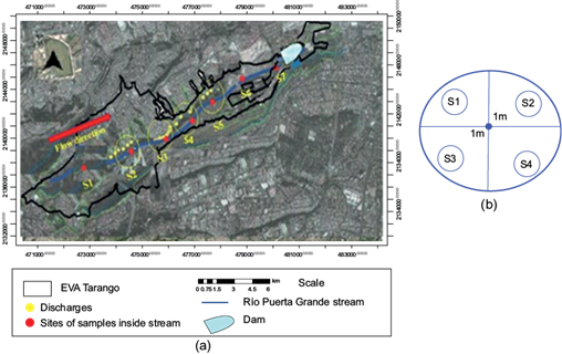
Fig. 2 (a) Discharge points and sample sites on the Río Puerta Grande stream. (b) Four-point sample pattern for each site.
The yellow points indicate locations where wastewater from communities above is discharged into the ravine. Sites S2 to S5 had the greatest wastewater discharge, and the red dots are the sampling sites along the stream. Water residue discharge mostly dominates during the dry season. Site S1 is in the upper part of the channel and is in a wooded area with no population. The stream runs inside the ravine and little sunlight penetrates through it. Sites S6 and S7 are completely outside the ravine and fully receive sunlight.
Physical, chemical, and biological analyses
Sampling from the seven sites along the stream were collected in 2020 during the dry season (specifically during February-March) and after the rainy season (October-November). The sampling followed the protocols established in the Mexican Standard NOM-001-SEMARNAT-1996 (SEMARNAT 1996). The temperature, pH, conductivity (Cond), and oxidationreduction potential (ORP) were simultaneously monitored in situ with Vernier LabQuest LABQ equipment, which was coupled to calibrated electrodes and used the following Mexican Standards: NMX-007-SCFI-2013 (SCFI 2013), for temperature; NMX-AA-008-SCFI-2016 (SCFI 2016), for pH; NMX-AA-093-SCFI-2000 (SCFI 2000), for conductivity; there are no regulations in Mexico for ORP. The dissolved oxygen (DO) was monitored with YSI 55 equipment by following Mexican Standard NMX-AA-012-SCFI-2001 (SCFI 2001d).
Regarding the ex-situ parameters, alkalinity (Alk) was determined according to Mexican standard NMX-AA-036-SCFI-2001 (SCFI 2001b) with VELP Scientifica equipment, Model FOC225E. To determine the water hardness (Hard) at each site, the following formula was used (represented by Equation 2 (Sawyer et al. 2001):
The biochemical oxygen demand (BOD) for this stream was analyzed by following Mexican Standard NMX-AA-028-SCFI-2001 (SCFI 2001e) and using VELP Scientifica equipment, Model FOC225E. The nitrate analysis (N-NO3-) was carried out using the DREL/2400 Complete Water Quality Laboratory equipment from Hach, following Mexican Standard NMX-AA-079-SCFI-2001 (SCFI 2001c). For the phosphate determination (P-PO4 3-) in the laboratory, Mexican Standard NMX-AA-029-SCFI-2001 (SCFI 2001a) was applied. Fecal coliform (FC) was determined according to Mexican Standard NMX-AA-042-SCFI-2015 (SCFI 2015). Total suspended solids (TSS) were determined at each site following Mexican Standard NMX-AA-034/2-SCFI-2008 (SCFI 2008).
Inverse distance weighted (IDW) interpolation
Information from topographic maps was obtained for the Tarango micro-basin. The basin has an uneven topography, and favors rapid water runoff. For this study, a geographic information system (GIS) was used to structure and visualize the topographical characteristics, land use, public service networks, and demographics (Najera et al. 2010). To establish the distribution of each parameter that applies to the stream, inverse distance weighted (IDW) interpolation was used via ArcGIS software. The maps were built with a raster format having a 5 m spatial resolution, which was produced through the ArcMap program. Equations 1 and 3 were used for the IDW interpolator (Ogbozige et al. 2018):
where:
λi |
is the weight of neighbor i |
d (So, Si) |
is the distance by which So and the Si are detached |
β |
is the coefficient used to adjust the weights |
n |
is the total number of sites in the neighborhood analysis |
Maps showing the spatial distribution of the parameters are useful for evaluating water quality and managing and distributing water resources.
Determination of the Río Puerta Grande stream quality indices
Analytical results of the parameters for each season (dry season and after the rainy season) were used: T, pH, TSS, Cond, Alk, Hard, DO, BOD, N-NO3-, P-PO43-, and FC. Table I shows the equations that were developed for each WQI, where the characteristics, comparison, and rating scales that were used to obtain the WQI for the two models used are indicated. Each quality level and numerical interval is represented with contrasting colors.
TABLE I RELATIONSHIP OF QUALITY INDICES AND RATING SCALE.
| Water Quality Index (WQI) | Equation | Characteristics | Grading Scale | |
| Montoya et al. (1997) |
|
Qi = quality index for the parameter and subscript of i-th parameter Wi = weighting coefficient of parameter i n = number of subscripts | QWI | Grading Scale |
| Not contaminated | 85-100 | |||
| Acceptable | 70-84 | |||
| Little contaminated | 50-69 | |||
| Contaminated | 30-49 | |||
| Highly contaminated | 0-25 | |||
| León (1992) Dinius (1987) |
|
Qi = subscript of i-th parameter Wi = weight or percentage assigned to the i-th parameter n = number of subscripts | QWI | Grading Scale |
| Excellent | 91-100 | |||
| Good | 71-90 | |||
| Medium | 51-70 | |||
| Bad | 26-50 | |||
| Very Bad | 0-25 | |||
Table II shows the equations used for each parameter in the two WQI models, where Ii and Qi are the quality functions for each of the parameters detailed by Montoya et al. and León-Dinius, respectively. In addition, i is i-th parameter.
TABLE II EQUATIONS USED TO CALCULATE Ii AND Qi ACCORDING TO MONTOYA et al. AND LEÓN-DINIUS.
| WQI (Montoya et. al. 1997a) WQI León (1992a), Dinius (1972a) |
|
|
| Hydrogen potential (pH) |
| Qi = 10(4.22 - 0.293pH) |
| Conductivity (COND) |
| Qi = 540 × CE(-0.379) |
| Alkalinity (ALK) |
| Qi = (105 × ALK)(-0.186) |
| Hardness (HARD) |
| Qi = 10(1.974 - (0.00174 × HARD)) |
| Dissolved Oxygen (DO) |
|
|
| Biochemical Oxygen Demand (BOD) |
| Qi = 120 × BOD(-0.673) |
| Nitrates (NO3-) |
| Qi = 162.2 × (NO3-)(-0.0343) |
| Phosphates (PO43-) |
| Qi = 34.215 × (PO43-)(-0.046) |
| Fecal coliforms (FC) |
| Qi = 97.51 × [5 × FC(-0.27)] |
| Total Suspended Solids (TSS) |
| Qi = 97.51 × [5 × FC(-0.27)] |
In table IIIa and table IIIb, the weights for each model are presented.
TABLE III WEIGHTING FACTOR TABLE FOR EACH PARAMETER: (a) ACCORDING TO MONTOYA et al. AND (b) ACCORDING TO LEÓN-DINIUS.
| WQI (Montoya et al. 1997a) | WQI León (1992a), Dinius (1972a) | ||
| Parameters | Weight (Wi) | Parameters | Weight (Wi) |
| Biochemical Oxygen Demand (BOD) | 5 | Biochemical Oxygen Demand (BOD) | 0.24016 |
| Dissolved Oxygen (DO) | 5 | Dissolved Oxygen (DO) | 0.20830 |
| Fecal coliforms (FC) | 5 | Fecal coliforms (FC) | 0.20830 |
| Conductivity (COND) | 2 | Conductivity (COND) | 0.08330 |
| Nitrates (NO3-) | 0.5 | Nitrates (NO3-) | 0.02083 |
| Phosphates (PO43-) | 0.5 | Phosphates (PO43-) | 0.20830 |
| Alkalinity (Alk) | 1 | Alkalinity (Alk) | 0.04166 |
| Hardness (HARD) | 1 | Hardness (HARD) | 0.04166 |
| Hydrogen potential (pH) | 1 | Hydrogen potential (pH) | 0.04166 |
| Total Suspended Solids (TSS) | 3 | Total Suspended Solids (TSS) | 0.08330 |
| Total | 24 | Total | 1.00000 |
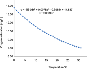
To calculate the DO and to apply the equations given in table IV, the DO saturation was first calculated by obtaining Equation 4 through a third-order polynomial curve (Fig. 3). The curve was constructed based on the DO concentration at the temperature noted and normal atmospheric pressure, which were obtained from the following relationship:
TABLE IV VALUES OF THE OXYGEN SATURATION IN FRESHWATER.
| Temperature (ºC) | DO (mg/L) | Temperature (ºC) | DO (mg/L) |
| 0 | 14.5 | 16 | 9.9 |
| 1 | 14.2 | 17 | 9.7 |
| 2 | 13.8 | 18 | 9.6 |
| 3 | 13.5 | 19 | 9.3 |
| 4 | 13.1 | 20 | 9.1 |
| 5 | 12.8 | 21 | 8.9 |
| 6 | 12.5 | 22 | 8.7 |
| 7 | 12.1 | 23 | 8.6 |
| 8 | 11.8 | 24 | 8.4 |
| 9 | 11.6 | 25 | 8.3 |
| 10 | 11.13 | 26 | 8.1 |
| 11 | 11.00 | 27 | 8.00 |
| 12 | 10.80 | 28 | 7.8 |
| 13 | 10.50 | 29 | 7.7 |
| 14 | 10.30 | 30 | 7.6 |
| 15 | 10.10 | 31 | 7.5 |
Water quality indices from Montoya et al. 1997
In Mexico, to indicate the quality of a body of water, the water quality index (WQI) from Montoya et al. (1997) is used. With this index, water quality is determined through an analysis of the physical, chemical, and bacteriological parameters, thus establishing the degree of contamination that exists in the water at the time of sampling, which is expressed as a percentage of pure water. This index considers a total of 18 parameters for its calculation, with different relative weights (Wi) being determined depending on the importance given to each of them in the total evaluation. In this work, the WQI of Montoya et al. (1997) was utilized by incorporating 10 parameters: pH, TSS, EC, Alk, DT, DO, BOD, N-NO3-, P-PO43 and FC.
Water quality indices from León 1991 and Dinius 1987
This index groups the most representative polluting variables. It is a model adapted from Dinius (1987). It considers multiplicative and weighted techniques (i.e., weighted geometric average), and is also useful for surface waters. The importance of the model lies in the fact that, given the scarcity of sample data and in the absence of some parameter values, its weight can be distributed proportionally among those that have been determined. In addition, the least important parameter can be excluded from the multiplicative operator when performing the global calculation for the WQI of the water subject under evaluation, but it still accommodates values allowed by the existing standard.
RESULTS AND DISCUSSION
The spatial distribution of each parameter was determined; then, the water quality index per site and for the overall stream were obtained. Two indices were used: Montoya et al. (1997) and León (1991), and these indices were used to compare and evaluate the environmental condition along reaches of the stream.
The spatial distribution of temperature along the stream
Temperature affects the solubility of dissolved gases in water and most biological processes in aquatic ecosystems. Water temperature varies due to changes in the natural environment that occur during each season of the year. At the studied site, its decrease was observed down to the deepest zone in which little sunlight is able to penetrate during either season. This parameter is important since at low temperatures there is a slow degradation of contaminants, especially bacteriological and organic matter. In figure 4a and figure 4b, the temperature distribution at the different sites in the two seasons are presented. Following the direction of the flow, the figure starts with the temperatures, represented in light green, for the sites S1 and S2; i.e., both showed 15.40-16.35 ºC in the dry season. After the rainy season, however, it was 13.74-14.51ºC for site S1 and 14.52-15.30 ºC for site S2 (shown in a yellow-green color), which is also where a decrease in this parameter was observed. At sites S3 to S5, the temperatures ranged between 13.48 and 14.44 ºC in the dry season and 12.16 and 12.94 ºC after the rainy season.
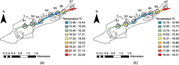
Fig. 4 Temperature distribution at the seven sites along the stream: (a) dry season; (b) after the rainy season.
These sites are in the deep end of the ravine, where little sunlight reaches (indicated in blue). Once the flow begins to exit the ravine, there is an increase in temperature at site S6, where temperatures of 17.32-18.26 ºC (yellow) were recorded downstream in the dry season and 16.09-16.86 ºC (orange) recorded after the rainy season. Site S7, which is located outside the ravine and where the sun’s rays fully reach the water, the temperatures were 21.14-22.09 ºC in the dry season and 18.44-19.21 ºC after the rainy season (red). Mexican Standard NOM-001-Semarnat-2021 accepts a maximum of a 35 ºC daily average for urban use. In both periods, this parameter did not exceed the limit.
pH spatial distribution along the stream
According to the maps shown in figure 5a, b, the pH distribution indicates that, as the flow of water flows along the ravine, the pH values at sites S1 and S2 ranged between 8.25 and 8.35 (shown in light orange) along the dry season. However, the pH ranges between 7.79 and 7.95 (light green, light orange, and orange) after the rainy season. At sites S2 and S3, it ranged from 7.96 to 8.00 (orange) after the rainy season, as indicated by the color change in each map. The values from sites S3 to S5 were 8.60-8.70 (light red) in the dry season. At sites S4 and S5, the values ranged between 7.90 and 7.95 (light orange) after the rainy season.
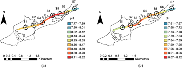
Fig. 5 The pH distribution at the seven sites along the stream: (a) dry season; (b) after the rainy season.
At site S6, the pH was 8.25-8.35 during the dry season, and after the rainy season it ranged from 7.84 to 7.89 (yellow). Finally, at site S7, the pH values were 7.90-8.01 in the dry season, and 7.68-7.72 after the rainy season (light blue). Generally, the values rose during the dry season throughout the stream, with an average of 8.33 ± 0.29. These values may indicate the predominance of bicarbonate, as this basicity can be caused by the degradation of organic matter (humic material).
Concerning the subsequent period following the rainy season, the pH decreased to 7.86 ± 0.14. According to Barrera et al. (2008), hydrolysis by organic material degradation influences the acidity together with the acidic rain that falls in Mexico City. As such, the temperature and pH are the main factors involved in the process. According to Henze et al. (2002), pH between 7.50 and 8.60 is ideal for nitrification, which is a process that lowers alkalinity by reducing the pH. Mexican Standard NOM-001-SEMARNAT-2021 (SEMARNAT 2021) considers permissible pH values those between 6 and 9; thus, this parameter was within the limits in the stream during both seasons.
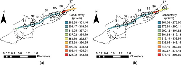
Conductivity spatial distribution along the stream
Electrical conductivity, which is the ability of water to conduct an electrical current, is directly related to the concentration of dissolved salts in a body of water. According to figure 6a, which corresponds to the dry season, the increase in conductivity is noted, and one of the causes for it was the discharge of community wastewater. In the dry season, the conductivity values at site S1 ranged between 283.68 and 301.46 µS/cm (light blue). For sites S2 to S5, the range in values was 301.47-319.24 µS/cm (blue). The S6 site increased to 408.14-425.91 µS/cm, where the dissolved ions were possibly concentrated from the wastewater discharged from the other sites. However, at site S7, it decreased to 372.58-390.35 µS/cm (light orange); at this site, there are no wastewater discharges because there is no population. Concerning after the rainy season period (Fig. 6b), the values decreased because of dilution; thus, from site S1 to S5, the interval was 261.08-275.60 µS/cm (blue), as in the previous case, and an increase of 377.19-391.69 µS/cm (deep red) was observed at site S6. Site S7 indicated in yellow-green, revealed a 304.63-319.13 µS/cm range.
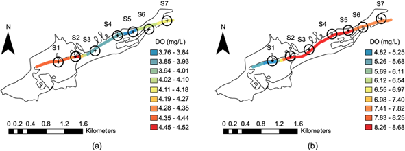
Dissolved oxygen spatial distribution along the stream
Dissolved oxygen (DO) is a critical parameter for aquatic ecosystems when its concentration ranges between 5 and 6 mg/L (Gómez et al. 2006). The Ecological Criteria for Water Quality CE-CCA-001/89 in Mexico establishes a minimum limit of 5 mg/L for the protection of aquatic life in both freshwater and marine water (SEDUE 1988). Some of the DO in water comes from the atmosphere, and after its dissolution at the water surface, the oxygen is distributed by currents and turbulence. Algae and aquatic plants also release oxygen to the water through photosynthesis (Manahan 2005). In our investigation, the increase in organic waste was the main factor contributing to the changes in dissolved oxygen levels. The decay of organic waste consumes oxygen (Manahan 2005), and the temperature, pressure, and salinity affect the ability of water to dissolve oxygen. Figure 7a shows this for the dry season, when a higher concentration was noted at sites S1 and S2 (bright orange); however, DO improved somewhat at site S1 in the rainy season (bright blue), as shown in Figure 7b. In the dry season, the values decreased at sites S3 to S5 (bright blue), which is where the most significant municipal discharges occur, meaning that the presence of organic matter consumes more DO. The DO improves from sites S6 and S7 (light green to yellow). The above is because, at these sites, there is no population. Therefore, there is no municipal discharge. After the rainy season, the DO increased from sites S2 to S7 (Fig. 6b), meaning the organic matter was dissolved.
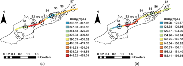
Spatial distribution of biochemical oxygen demand along the stream
Biochemical oxygen demand (BOD) indicates the water quality relative to the organic matter that is present and measures how much oxygen is consumed for purification. The higher the BOD concentration, the greater the amount of degradable organic matter. As such, this parameter is used as an indicator of the organic load that is discharged by wastewater effluents. For surface waters, it is an indicator associated with microbial respiration processes (Fig. 8a). This conditions corresponds to the dry season, when the water origin is fully residual. The highest BOD concentration occurred in sites S2 and S3 (red), which implies that at these sites there is greater oxidation of organic matter. The BOD concentration decreases at site S4, but increases again at sites S5, S6 and S7. In the period after the rainy season (Fig. 8b) there is a decrease in BOD that is associated with dilution. At site S1 the decrease is 67.00%, at sites S2 to S3 the decrease is 61.81%, and at sites S5 to S6 the decrease is 66.62% (Fig. 8a, b). Mexican Standard NOM-001-SEMARNAT-1996 (SEMARNAT 1996) sets a maximum daily average limit of 150 mg/L for urban use; therefore, the values during both seasons exceeded this limit.
Alkalinity spatial distribution along the stream
Alkalinity is essential in water bodies; it is the primary buffer system in freshwater and the productivity of natural water bodies, and it is considered a reserve source for the photosynthesis of aquatic plants and algae. It is closely related to pH and hardness since alkalinity is due to bicarbonates and carbonates. It is also a component of carbonated hardness (temporary hardness). Figure 9 shows that all the recorded pH values ranged between 8.7 and 7.6, which indicates that bicarbonate determines the alkalinity. In the dry season (Fig. 9a) at site S1, the values ranged between 207 and 135 mg/L in CaCO3 units, where the lowest values are shown in bright blue. Site S6 had the highest values, between 197.27 and 207.55 mg/L (light red). In the period after the rainy season (Fig. 9b), the values decreased to around 55.15% between the lowest values at site S1 (blue) and 56.62% between the highest values at site S6 (red).
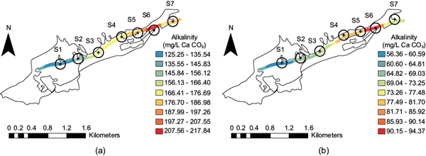
Fig. 9 Alkalinity distribution along the stream at the seven sites: (a) dry season; (b) after the rainy season.
According to data from CONAGUA (2022), there was abundant rainfall in 2020 (in mm): May, 32.8; June, 59.7; July, 103.8; August, 107.8; September, 97.0; and October, 20.1. Thus, this decrease in alkalinity was attributed to dilution. According to Pérez (2016) (who quotes Ramalho 2003), in domestic wastewater there is 250 mg/L in CaCO3 units. In the case of the stream, the values were smaller (mainly in the dry season).
Hardness spatial distribution along the stream
Neira (2006) mentions that geological factors mainly control water hardness. The primary mineral sources of hardness come from the soil, and the water will be hard according to the soil composition. Hard water is concentrated in calcium and magnesium and is associated with sedimentary rock catchments, the most common of which are limestone and chalk. The Tarango micro-basin comprises Miocene andesitic and dacite volcanic rocks, intercalated pumice sand deposits, altered tuffs, pumice horizons, and clayey soils. The water in the stream is hard, according to the hardness classification. During both seasons, the values were slightly different, increasing more after the rainy season since more calcium and magnesium ions could be desorbed from the suspended material and by erosion of the ravine soil. It can be seen from figure 10a and figure 10b that site S3 presented the highest value (red), 272.92-284.47 mg/L in CaCO3 units in the dry season and 282.61-295.88 mg/L in CaCO3 units after the rainy season.
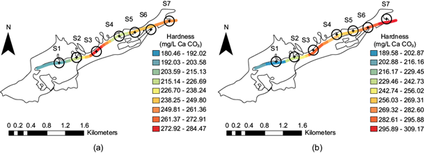
Fig. 10 Hardness distribution at the seven sites along the stream: (a) dry season; (b) after the rainy season.
During the dry season, site S2 presented values between 226.70 and 238.24 mg/L in CaCO3 units (yellow), which decreased following the rainy season to between 229.46 and 242.73 mg/L in CaCO3 units (light green). At site S4, the range 226.70-238.24 mg/L in CaCO3 units (yellow) was observed in the dry season. After the rainy season, this increased to between 256.03 and 269.31 mg/L in CaCO3 units (light orange). At sites S5 and S6, values between 238.25 and 249.80 mg/L in CaCO3 units (light orange) were recorded in the dry season. At site S7 in the dry season the range is 249.81 to 261.36 mg/L CaCO3 units (bright orange), but it increased after the rainy season from 295.89 to 309.17 mg/L CaCO3 units (red) (Fig. 10a, b). This increase occurs despite the dilution that occurs after the rainy season.
According to the U.S. Geological Survey (USGS 2018), the following classification for hard and soft water is used: 0 to 60 mg/L, in CaCO3 units, is classified as “soft”; 61 to 120 mg/L, in CaCO3 units, is “moderately hard”; 121 to 180 mg/L, in CaCO3 units, is “hard”; and more than 180 mg/L, in CaCO3 units, is classified as “very hard”. Therefore, the water of this stream was considered very hard.
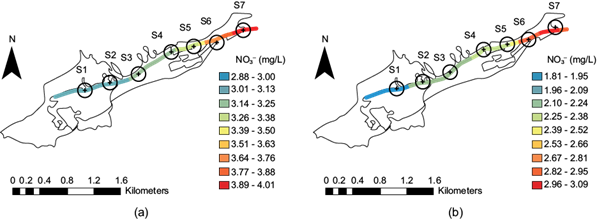
Nitrate spatial distribution along the stream
The presence of nitrate in water bodies is a problem; nitrate can be present because of the dissolution of rocks that contain it or from wastewater discharges. Its concentration in uncontaminated water is highly variable, although it does not usually exceed 10 mg/L (Brenes et al. 2011). Runoff following the use of nitrogenous fertilizers is another contribution. In this study, the concentration was generally not high during both periods. In the period after the rainy season, however, it decreased to approximately 40%. In both periods, the highest concentration was observed at sites S6 and S7 (indicated by colors between light green and yellow) in figure 11a and figure 11b. In general, from sites S3 to S5, there are residual discharges that increase the presence of nitrate. In this stream, due to the shallow water depth (0.25 m), the presence of DO, and the rapid water flow, no ammoniacal nitrogen or nitrites were detected.
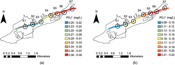
Phosphate spatial distribution along the stream
Phosphate (P-PO43-) in this micro-basin, at least in the year in which the samplings were carried out, had a particularly low concentration; in the period after the rainy season, it was much less. By analyzing figure 12a, in the dry season the concentration at site S3 ranges between 0.27 and 0.28 mg/L (green light) and increases at site S4 between 0.29 and 0.31 mg/L (yellow). In the period after the rainy season (Fig. 12b), the concentration at these sites decreased almost 50%. Therefore, sites S3 and S4 ranged from 0.16 mg/L (yellow) and up to 0.17 mg/L (light orange), respectively. During both periods, sites S5, S6, and S7 presented the highest concentration concerning the other sites. In the dry season at sites S5, S6, and S7, the concentration ranges from 0.38 to 0.39 mg/L (Fig. 12a), and after the rainy season, from 0.21 to 0.22 mg/L (Fig. 12b). For phosphate, Mexican Standard NOM-001-SEMARNAT-2021 (SEMARNAT 2021) sets a daily average limit of 18 mg/L for urban use. Furthermore, the values found in the stream did not even reach 1 mg/L, as the highest concentration was 0.39 mg/L.
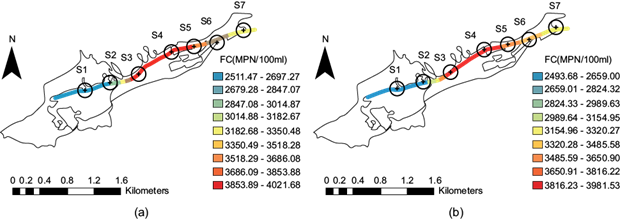
Fecal coliform spatial distribution along the stream
Concerning fecal coliform, the average values analyzed were well above the permissible levels indicated by Mexican Standard NOM-001-SEMARNAT-1996 (SEMARNAT 1996), which lists the permitted limit as 250 MPN/100 mL. It was observed that samples collected during both periods, as shown in figure 13a and figure 13b, exceeded this limit, and the samples’ values were similar for both periods. Figure 13 shows that acute risk was present throughout the entire channel, and its control was prioritized through specific treatment systems. The high values of 3853.89-4021.68 MPN/100 mL and 3816.23-3981.53 MPN/100 mL are mainly due to municipal discharge. We observed high values (dark red) at sites S3 to S4 during both periods. We observed high values (dark red) at sites S3 to S4 during both periods. There is a slight decrease in the concentration of fecal coliforms at site S5; this is probably associated with a lower population density that discharges its wastewater into the stream at this site. Concerning fecal coliform, the average values analyzed were well above the levels according to NOM-001-SEMARNAT (SEMARNAT 1996), where the maximum permissible limit is 1000 and 2000 fecal coliform per 100 mL per day for wastewater discharge into national waters.
Total suspended solids spatial distribution along the stream
Total suspended solids (TSS) are particularly important because they have porous surfaces that can adsorb chemical species such as cations and anions. The clayey material is a support for organic matter. This phenomenon is extremely important for transport studies, so it was necessary to measure the concentration of this material at the four points for each of the seven sites, both during the dry season and after the rainy season. Figure 14a and figure 14b show that each point per site was heterogeneous, which is interesting for studies on the hydrodynamics of the stream and, therefore, for transport since suspended solids provide surfaces that sequester metals. As the flow advances, more material is eroded and suspended, which was observed more in the period after the rainy season. Figure 14a shows that the highest concentration occurred at site S7 1057.09-1096.23 mg/L, (red) for both periods.
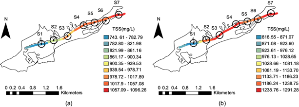
Fig 14 Total suspended solids distribution along the stream at the seven sites: (a) dry season; (b) after the rainy season.
In contrast to the other parameters, in the case of the period after the rainy season (Fig. 14b) the concentration was 1238.76-1296.28 mg/L at sites S3 and S4 (red) due to the erosion and suspension by the water flow. This fell to 1133.71-1186.23 mg/L at site S5 (orange), rising to 1186.24-1238.75 mg/L (light red) at site S6, and ending with a concentration of 1238.76-1291.28 mg/L (dark red) at site S7. Mexican Standard NOM-001-SEMARNAT-2021 sets a daily average limit of 72 mg/L for urban use.
The water quality index (WQI) determination of each site at the Río Puerta Grande stream
The results for Ii and Qi (Table V and Table VI) for the two WQI models are presented with each of the physical and chemical parameters that contributed to the Río Puerta Grande stream quality index. Using the equations for the calculation from table II that correspond to two sampling seasons, i.e., the dry season and after the rainy season, four points for each of the seven sites were measured. Table IV indicates the standard deviation for each value of Qi per site.
TABLE V Qi RESULTS (QUALITY INDEX FOR THE PARAMETER AND SUBSCRIPT OF THE i-th PARAMETER) FOR THE MONTOYA et al. WQI MODEL.
| Sites | Qi in Dry season (Montoya et al., 1997) | |||||||||
| pH | COND | ALK | HARD | DO | BOD | NO3- | PO43- | FC | TSS | |
| S1 | 57.77 ± 2.58 | 65.31 ± 0.28 | 84.80 ± 0.68 | 39.53 ± 0.30 | 220.72 ± 5.51 | 11.04 ± 0.02 | 27.78 ± 0.33 | 16.00 ± 0.30 | 38.14 ± 0.10 | 68.55 ± 1.04 |
| S2 | 56.24 ± 2.82 | 65.29 ± 0.11 | 82.73 ± 0.50 | 38.48 ± 0.40 | 218.25 ± 2.00 | 9.72 ± 0.09 | 27.73 ± 0.35 | 17.88 ± 0.26 | 37.59 ± 0.18 | 65.85 ± 1.14 |
| S3 | 48.48 ± 2.53 | 65.09 ± 0.19 | 82.66 ± 0.35 | 36.83 ± 0.13 | 187.93 ± 9.08 | 11.88 ± 0.12 | 27.31 ± 0.25 | 15.93 ± 0.29 | 34.02 ± 0.07 | 62.53 ± 0.73 |
| S4 | 45.32 ± 1.26 | 65.02 ± 0.28 | 80.48 ± 0.49 | 38.28 ± 0.08 | 186.46 ± 2.44 | 10.52 ± 0.18 | 27.15 ± 0.18 | 14.78 ± 0.28 | 33.74 ± 0.09 | 62.20 ± 0.64 |
| S5 | 45.01 ± 2.63 | 65.02 ± 0.16 | 79.49 ± 0.32 | 37.76 ± 0.24 | 182.62 ± 2.27 | 10.38 ± 0.14 | 26.84 ± 0.16 | 13.55 ± 0.28 | 33.73 ± 0.10 | 62.16 ± 0.47 |
| S6 | 59.76 ± 4.28 | 56.41 ± 0.27 | 77.39 ± 0.28 | 37.66 ± 0.10 | 220.18 ± 4.15 | 10.36 ± 0.06 | 25.79 ± 0.26 | 13.33 ± 0.13 | 35.01 ± 0.11 | 61.55 ± 0.14 |
| S7 | 77.22 ± 9.31 | 61.18 ± 0.24 | 79.91 ± 0.36 | 37.50 ± 0.17 | 234.45 ± 3.60 | 10.36 ± 0.07 | 25.31 ± 0.68 | 13.40 ± 0.13 | 34.87 ± 0.05 | 60.28 ± 0.27 |
| Sites | Qi After rainy season (Montoya et al., 1997) | |||||||||
| pH | COND | ALK | HARD | DO | BOD | NO3- | PO43- | FC | TSS | |
| S1 | 87.78 ± 5.39 | 62.20 ± 0.50 | 98.38 ± 0.78 | 39.27 ± 0.29 | 237.17 ± 5.06 | 23.77 ± 0.35 | 32.77 ± 0.30 | 25.82 ± 0.63 | 38.03 ± 0.10 | 66.68 ± 0.26 |
| S2 | 76.70 ± 6.27 | 61.46 ± 0.26 | 95.98 ± 0.58 | 38.24 ± 0.42 | 242.27 ± 1.94 | 19.33 ± 0.15 | 31.59 ± 0.54 | 22.62 ± 0.21 | 37.50 ± 0.25 | 57.37 ± 0.07 |
| S3 | 77.74 ± 3.36 | 60.86 ± 0.24 | 95.57 ± 0.42 | 36.48 ± 0.08 | 198.90 ± 9.08 | 19.84 ± 0.19 | 31.01 ± 0.41 | 20.37 ± 0.29 | 33.90 ± 0.03 | 56.65 ± 0.10 |
| S4 | 78.80 ± 2.36 | 60.76 ± 0.28 | 92.98 ± 0.57 | 37.38 ± 0.15 | 198.10 ± 7.54 | 21.56 ± 0.52 | 30.72 ± 0.24 | 18.82 ± 0.38 | 33.62 ± 0.05 | 56.55 0.24 |
| S5 | 79.87 ± 1.47 | 60.53 ± 0.19 | 92.84 ± 0.38 | 37.20 ± 0.40 | 195.60 ± 1.98 | 22.19 ± 0.25 | 30.55 ± 0.29 | 17.44 ± 0.40 | 34.03 ± 0.10 | 59.13 ± 0.34 |
| S6 | 84.30 ± 4.95 | 53.79 ± 0.23 | 90.41 ± 0.33 | 36.79 ± 0.25 | 221.77 ± 4.47 | 21.18 ± 0.11 | 32.77 ± 0.30 | 17.78 ± 0.37 | 34.92 ± 0.20 | 57.58 ± 0.11 |
| S7 | 92.65 ± 5.91 | 57.19 ± 0.20 | 95.32 ± 0.43 | 36.31 ± 0.17 | 232.05 ± 3.76 | 21.85 ± 0.53 | 31.59 ± 0.54 | 17.93 ± 0.35 | 35.55 ± 0.12 | 56.79 ± 0.22 |
TABLE VI Qi RESULTS (QUALITY INDEX FOR THE PARAMETER AND SUBSCRIPT OF i-th PARAMETER) FOR THE LEÓN-DINIUS WQI MODEL
| Sites | Qi in Dry Season (León (1991a, Dinius (1987) | |||||||||
| pH | COND | ALK | HARD | DO | BOD | NO3- | PO43- | FC | TSS | |
| S1 | 57.77 ± 2.58 | 65.31 ± 0.28 | 42.40 ± 0.34 | 39.52 ± 0.30 | 44.14 ± 1.10 | 2.21 ± 0.03 | 111.11 ± 1.32 | 63.99 ± 1.20 | 58.89 ± 0.15 | 22.85 ± 0.35 |
| S2 | 56.24 ± 2.83 | 65.29 ± 0.11 | 41.37 ± 0.25 | 38.48 ± 0.40 | 43.65 ± 0.40 | 1.94 ± 0.02 | 110.93 ± 1.38 | 71.51 ± 1.04 | 58.05 ± 0.28 | 21.95 ± 0.38 |
| S3 | 48.48 ± 2.53 | 65.08 ± 0.19 | 41.33 ± 0.18 | 36.83 ± 0.13 | 37.59± 1.82 | 1.99 ± 0.02 | 109.23 ± 0.99 | 63.73 ± 1.18 | 52.53 ± 0.12 | 20.84 ± 0.24 |
| S4 | 45.32 ± 1.26 | 65.02 ± 0.28 | 40.24 ± 0.25 | 38.28 ± 0.08 | 37.29± 0.49 | 2.38 ± 0.03 | 108.59± 0.71 | 59.10 ± 1.14 | 52.11 ± 0.14 | 20.73 ± 0.22 |
| S5 | 45.01 ± 2.63 | 65.02 ± 0.16 | 39.75 ± 0.16 | 37.38 ± 0.15 | 36.52 ± 0.45 | 2.10 ± 0.02 | 107.37 ± 0.66 | 54.22 ± 1.13 | 52.09 ± 0.15 | 20.72 ± 0.16 |
| S6 | 59.76 ± 4.28 | 56.41 ± 0.27 | 38.69 ± 0.14 | 37.76 ± 0.24 | 44.04 ± 0.83 | 2.08 ± 0.01 | 103.14 ± 1.05 | 53.31 ± 0.55 | 54.06 ± 0.17 | 20.52 ± 0.05 |
| S7 | 77.22 ± 9.31 | 61.18 ± 0.24 | 39.96 ± 0.18 | 37.50 ± 0.17 | 46.89 ± 0.32 | 2.07 ± 0.01 | 101.25 ± 0.64 | 53.61 ± 0.50 | 53.85 ± 0.07 | 20.09 ± 0.09 |
| Sites | Qi After Rain (León (1991a), Dinius (1987) | |||||||||
| pH | COND | ALK | HARD | DO | BOD | NO3- | PO43- | FC | TSS | |
| S1 | 87.78 ± 5.39 | 62.20 ± 0.50 | 49.188 ± 0.39 | 39.26 ± 0.29 | 47.43 ± 1.01 | 4.75 ± 0.07 | 131.82 ± 1.21 | 103.29 ± 2.50 | 58.73 ± 0.16 | 22.23 ± 0.09 |
| S2 | 76.70 ± 6.27 | 61.46 ± 0.25 | 47.988 ± 0.29 | 38.24 ± 0.42 | 48.45 ± 0.39 | 3.86 ± 0.03 | 126.38 ± 2.18 | 90.48 ± 0.85 | 57.91 ± 0.39 | 19.12 ± 0.02 |
| S3 | 77.74 ± 3.36 | 60.86 ± 0.23 | 47.786 ± 0.21 | 36.48 ± 0.08 | 39.78 ± 1.51 | 3.97 ± 0.04 | 124.03 ± 1.63 | 81.49 ± 1.14 | 52.34 ± 0.05 | 18.88 ± 0.03 |
| S4 | 78.80 ± 2.36 | 60.76 ± 0.28 | 46.492 ± 0.28 | 37.38 ± 0.15 | 39.62 ± 0.43 | 4.31 ± 0.10 | 122.90 ± 0.97 | 75.27 ± 1.51 | 51.92 ± 0.07 | 18.85 ± 0.08 |
| S5 | 79.87 ± 1.47 | 65.02 ± 0.19 | 46.422 ± 0.19 | 37.20 ± 0.40 | 39.12 ± 0.40 | 4.44 ± 0.05 | 122.19 ± 1.16 | 69.76 ± 1.61 | 52.56 ± 0.16 | 19.71 ± 0.11 |
| S6 | 84.30 ± 4.95 | 53.79 ± 0.23 | 45.208 ± 0.16 | 36.79 ± 0.25 | 44.35 ± 0.89 | 4.24 ± 0.02 | 114.81 ± 1.60 | 71.14 ± 1.47 | 53.93 ± 0.31 | 19.19 ± 0.04 |
| S7 | 92.65 ± 7.91 | 57.19 ± 0.20 | 47.657 ± 0.22 | 36.31 ± 0.17 | 46.41 ± 0.75 | 4.37 ± 0.02 | 111.79 ± 1.53 | 71.72 ± 1.41 | 54.89 ± 0.18 | 18.93 ± 0.07 |
Table VII presents the results of WQI calculations for the ten parameters. The weights assigned by the model in the two monitoring seasons are considered through the global model of Montoya et al. (1997). As the first step, each parameter was assigned a specific weight (Wi) according to its importance in terms of water quality for this stream. Moreover, Wi with the highest assigned hierarchies were also the most important parameters to consider; these parameters were DO, BOD, and fecal coliform as indicated in table IIb.
TABLE VII WQI VALUES FOR EACH PARAMETER AND THE OVERALL WQI.
| WQI | Sites | WQI Dry season parameters | ||||||||||
| pH | COND | ALK | HARD. | DO | BOD | NO3- | PO43- | FC | TSS | Overall WQI | ||
| Montoya, et al., (1997) | S1 | 2.41 | 3.66 | 1.77 | 1.65 | 1.84 | 0.09 | 4.63 | 2.67 | 6.59 | 0.95 | 26.25 |
| S2 | 2.34 | 3.20 | 1.72 | 1.60 | 1.82 | 0.08 | 4.62 | 2.98 | 6.49 | 0.91 | 25.78 | |
| S3 | 2.02 | 3.24 | 1.72 | 1.53 | 1.57 | 0.08 | 4.55 | 2.66 | 5.88 | 0.87 | 24.12 | |
| S4 | 1.89 | 3.28 | 1.68 | 1.60 | 1.55 | 0.10 | 4.52 | 2.46 | 5.83 | 0.86 | 23.78 | |
| S5 | 1.88 | 3.33 | 1.66 | 1.57 | 1.52 | 0.09 | 4.47 | 2.26 | 5.83 | 0.86 | 23.47 | |
| S6 | 2.49 | 3.51 | 1.61 | 1.57 | 1.83 | 0.09 | 4.30 | 2.22 | 6.05 | 0.85 | 24.53 | |
| S7 | 3.22 | 3.86 | 1.66 | 1.56 | 1.95 | 0.09 | 4.22 | 2.23 | 6.03 | 0.84 | 25.66 | |
| Sites | WQI After rain parameters | |||||||||||
| pH | COND | ALK | HARD. | DO | BOD | NO3- | PO43- | FC | TSS | Overall WQI | ||
| S1 | 3.66 | 2.72 | 2.05 | 1.64 | 1.98 | 0.20 | 5.49 | 4.30 | 6.57 | 0.93 | 29.53 | |
| S2 | 3.20 | 2.72 | 2.00 | 1.59 | 2.02 | 0.16 | 5.27 | 3.77 | 6.48 | 0.80 | 28.00 | |
| S3 | 3.24 | 2.71 | 1.99 | 1.52 | 1.66 | 0.17 | 5.17 | 3.40 | 5.86 | 0.79 | 26.49 | |
| S4 | 3.28 | 2.71 | 1.94 | 1.56 | 1.65 | 0.18 | 5.12 | 3.14 | 5.81 | 0.79 | 26.17 | |
| S5 | 3.33 | 2.71 | 1.93 | 1.55 | 1.63 | 0.18 | 5.09 | 2.91 | 5.88 | 0.82 | 26.04 | |
| S6 | 3.51 | 2.35 | 1.88 | 1.53 | 1.85 | 0.18 | 4.78 | 2.96 | 6.03 | 0.80 | 25.89 | |
| S7 | 3.86 | 2.55 | 1.99 | 1.51 | 1.93 | 0.18 | 4.37 | 2.99 | 6.14 | 0.79 | 26.31 | |
 Highly
contaminated
Highly
contaminated
Concerning the colors that indicate the quality of the water shown in table I, the total WQI (as per the Montoya et al. model) were black for all sites. In table VIII, the same calculation mechanism was carried out but with the model of León (1991) and Dinius (1987) being applied instead. Within this model, site S3 showed particularly poor results, and the other sites also demonstrated poor results for the period after the rainy season; furthermore, during the dry season, all the sites showed especially poor results.
TABLE VIII WQI VALUES FOR EACH PARAMETER AND THE OVERALL QWI.
| WQI | Sites | WQI Dry season parameters | ||||||||||
| pH | COND | ALK | HARD | DO | BOD | NO3- | PO43- | FC | TSS | Overall WQI | ||
| León (1992), Dinius (1987) | S1 | 1.18 | 1.42 | 1.17 | 1.17 | 2.20 | 1.22 | 1.10 | 1.09 | 2.34 | 1.30 | 22.37 |
| S2 | 1.18 | 1.42 | 1.17 | 1.16 | 2.20 | 1.18 | 1.10 | 1.09 | 2.33 | 1.29 | 21.46 | |
| S3 | 1.18 | 1.42 | 1.17 | 1.16 | 2.13 | 1.19 | 1.10 | 1.09 | 2.28 | 1.29 | 20.20 | |
| S4 | 1.17 | 1.42 | 1.17 | 1.16 | 2.13 | 1.24 | 1.10 | 1.09 | 2.28 | 1.29 | 20.93 | |
| S5 | 1.17 | 1.42 | 1.17 | 1.16 | 2.12 | 1.20 | 1.10 | 1.09 | 2.28 | 1.29 | 20.15 | |
| S6 | 1.19 | 1.40 | 1.16 | 1.16 | 2.20 | 1.20 | 1.10 | 1.09 | 2.30 | 1.29 | 20.97 | |
| S7 | 1.20 | 1.41 | 1.17 | 1.16 | 2.23 | 1.20 | 1.10 | 1.09 | 2.29 | 1.28 | 21.58 | |
| Sites | WQI After rain parameters | |||||||||||
| pH | COND | ALK | HARD. | DO | BOD | NO3- | PO43- | FC | TSS | Overall WQI | ||
| S1 | 1.20 | 1.41 | 1.18 | 1.17 | 2.23 | 1.48 | 1.11 | 1.10 | 2.34 | 1.29 | 28.35 | |
| S2 | 1.20 | 1.41 | 1.17 | 1.16 | 2.24 | 1.40 | 1.11 | 1.10 | 2.33 | 1.28 | 26.29 | |
| S3 | 1.20 | 1.41 | 1.17 | 1.16 | 2.15 | 1.41 | 1.11 | 1.10 | 2.28 | 1.28 | 24.72 | |
| S4 | 1.20 | 1.41 | 1.17 | 1.16 | 2.15 | 1.44 | 1.11 | 1.09 | 2.28 | 1.28 | 25.14 | |
| S5 | 1.20 | 1.42 | 1.17 | 1.16 | 2.15 | 1.45 | 1.11 | 1.09 | 2.28 | 1.28 | 25.52 | |
| S6 | 1.20 | 1.39 | 1.17 | 1.16 | 2.20 | 1.44 | 1.10 | 1.09 | 2.29 | 1.28 | 25.56 | |
| S7 | 1.21 | 1.40 | 1.17 | 1.16 | 2.22 | 1.45 | 1.10 | 1.09 | 2.30 | 1.28 | 26.34 | |
 Bad
Bad
 Very bad
Once each WQI per parameter and the total WQI were obtained, the colors listed in table I were used for demonstrating the final evaluation of the stream’s water quality. Figure 15a and figure 15b show the total WQI comparison for each model. It is observed that, with both models, the situation concerning the stream water quality was especially critical.
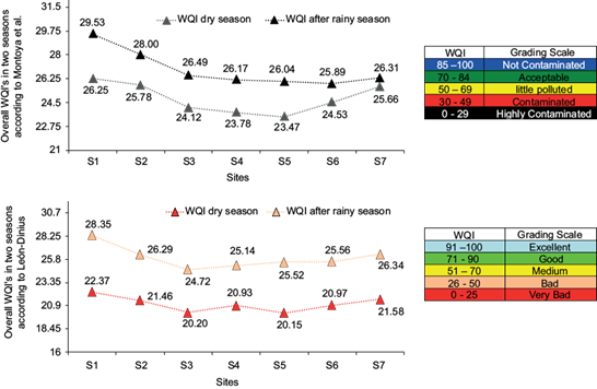
Fig. 15 Overall WQI of the Río Puerta Grande stream as per the Montoya et al. and León-Dinius models.
Both models and both seasons showed that the water, as per Montoya et al., were “Highly contaminated” (black) and, as per León-Dinius, “Bad” and “Very bad” (orange and red, respectively). However, although it improved slightly in the period after the rainy season, the quality continued to be critically poor.
CONCLUSIONS
According to the spatial distribution maps created using ArcGIS software for the seven sampling sites, the sites with high urban concentration experienced increased residual discharge in the dry season, and the concentration of parameters such as BOD and fecal coliform also increased. At this time, there was a decrease in dissolved oxygen resulting from the oxidation of organic matter. After the rainy season, other parameters such as BOD, nitrate, phosphate, and metals decreased due to a dilution effect. The fecal coliform concentrations were practically the same for the two periods. The fecal coliform levels were always above the limits detailed in Mexican Standard NOM-001-SEMARNAT-1996. The total solids in suspension increased during the period after the rainy season due to erosion caused by rains.
The importance of WQIs for the evaluation of water quality, since it allows for a determination of the degree of water purity or contamination, was demonstrated in this report. In addition, it is also useful for government authorities and civil society regarding the need to conserve or solve the problem presented by one water body.
As there are many water quality indices that are commonly used and which consider different variables, care must be taken when selecting the WQI to be used. Depending on the type of water body and its subsequent use, water can be used either for drinking water, recreation, industry, and/or agriculture.
The resulting evaluation of the stream according to the two WQI models is that its situation is critical, since the water was deemed to be “Highly contaminated” during both seasons. According to the evaluation method from León (1991) and Dinius (1987), the results were “Very bad” in the dry season, and “Bad” at sites S1, S2, S4, S5, S6, and S7 during the period after the rainy season (only site S3 was “Very bad” in this period). In general, the results of the WQI were consistent in terms of the extent of poor water quality. Deterioration was observed in the water quality of the stream due to the high BOD levels and FC, and the low levels of DO, which were due to discharges of domestic origin.

