


 nueva página del texto (beta)
 Inglés (pdf)
 Artículo en XML
 Referencias del artículo
 Enviar artículo por email
 Citado por SciELO
  Similares en
SciELO
Similares en
SciELO 
 Permalink
INTRODUCTION
The presence of pollutants in the environment is usually linked to wastes from anthropogenic activities, being oceans, rivers, and lakes the final destination of these products (Vareda et al. 2019). Heavy metals are among the most common contaminants since they are present in the Earth’s crust, manufactured products, and industrial wastes (Vareda et al. 2019). These elements have a negative impact in the environment since once they are in water bodies like reservoirs, they tend to adsorb in sediments (Meena et al. 2017). However, a percentage of these contaminants are bioavailable to biota present in the system, leading to adverse consequences for certain organisms (Ali and Khan 2018). Due to the negative effects of heavy metals in biota, different organizations like the United States Environmental Protection Agency (EPA) have created guidelines that set the maximum concentration limit in water bodies that provide services to humans like reservoir. For that reason, they should be monitored regularly as an early alert system; a way to do it is with bioindicators of pollution (Manickavasagam et al. 2019).
Bioindicators can accumulate a specific contaminant and reflect environmental conditions, making them a reliable tool for monitoring systems (Bonanno et al. 2018). Plants have been used as indicators of heavy metals by accumulation in other studies due to their natural history and their ability to accumulate these elements in different tissues (Bonanno et al. 2018). The advantage of using a bioindicator and not water is that the second only shows contaminant levels at a specific time. Unlike bioindicators, which accumulate the pollutant of interest over time, making analyses more robust (Manickavasagam et al. 2019). Additionally, the use of a bioindicator in most cases reduces sampling costs and effort, since some environmental data is not required to know the state of a certain study area.
Venezuela reservoirs like La Mariposa, Camatagua, and La Pereza are intervened with informal houses. Additionally, these areas usually lack of proper wastewater management (González and Ortaz 1998, González et al. 2003, Bentancourt and Mena 2012). On the other hand, the presence of plants like Eichhornia crassipes (water hyacinth) and Lemna minor (duckweed) has been reported in these reservoirs. These plants have properties that make them potential bioindicators of heavy metals. Both can accumulate and tolerate some metals such as Cu, Hg, Ni, Pb, and Zn (Bonanno et al. 2018). Additionally, their life cycle, size, and abundance make them potential bioindicators (Bonanno et al. 2018).
The study aims to determine the concentration of five metals in water and sediments of three reservoirs that provide services in Caracas, Venezuela, and evaluate the potential of water macrophytes E. crassipes and L. minor as bioindicators of heavy metals pollution by accumulation.
MATERIALS AND METHODS
Study area
La Mariposa
La Mariposa (LM; Fig. 1) is located in Miranda state and has a capacity of 8 million m3. Sportfishing and hiking activities are performed in the area. The tributaries of La Mariposa are El Valle river, Los Indios brook, and Camatagua and Lagartijo reservoirs. Slopes are affected by human activities and the lack of a proper sewer system (González et al. 2003, Bentancourt and Mena 2012). On the other hand, LM’s tributaries have an input of organic matter and fertilizers coming from farmhouses, pig houses and nurseries (González and Ortaz 1998). The dominant species in LM reservoir was E. crassipes and in a lower proportion was found L. minor.
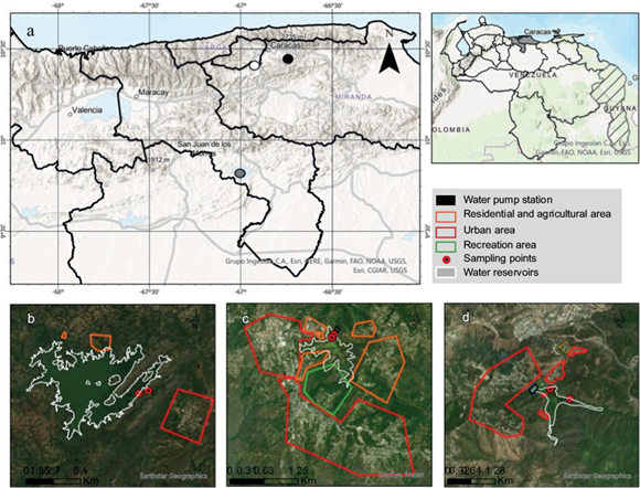
Camatagua
Camatagua (CM) is the biggest damn river in Venezuela, located in Aragua state (Fig. 1). It has a capacity of 1 573 million m3, being Guárico river its principal tributary. In the past, recreational activities were performed in the reservoir, nowadays these facilities are abandoned, and there is only the presence of sport fishermen. Slopes are also affected by human activities, informal houses, and some areas have been deforested (Bentancourt and Mena 2012). Likewise, during the sampling, it was observed that some slopes were affected by a recent fire. In the water, the dominant species was E. crassipes.
La Pereza
La Pereza (LP) is a compensatory reservoir located in Miranda state (Fig. 1). It has a capacity of 8 million m3, being La Pereza brook and other reservoirs from the Tuy system its principal tributaries. However, at the moment of the sampling, the rain was the only supply of LP. On the other hand, LP is highly intervened with livestock houses and farmhouses (González et al. 2003). The dominant species was Pistia stratiotes which cover the totality of the reservoir, except for the water pumps area, where L. minor was the dominant species.
Experimental design
There were three factors in the design, reservoir, sampling point, and transects. In each of the sampling points three transects were set, and in each transect three samples were collected, as specified in table I. Samples were collected between December 2018 and June 2019. The sampling points were in the shoreline of reservoirs and classified as entrance and exit (Fig. 1). CM’s entrance was a brook, and the exit was the Guárico river located outside the damn. LM’s entrance was the river mouth of Los Indios brook, and the exit was near the water outlet. LP’s entrance was the farthest point from the damn, and the exit was near the pumping station. On the other hand, sediments samples were collected using a steel collector at 6 m deep in LM’s exit and 3 m deep in LM’s entrance, and 0.5 m at LP and CM, and stored in polyethylene containers. Contrary to water samples which were from the surface and kept in polyethylene bottles. E. crassipes and L. minor were collected only in the sampling points where they were present as defined in table I. Additionally, they were washed with the reservoir’s water before being transported to the laboratory in plastic bags, where they were washed with distilled water and dissected in roots and leaves. Finally, they were stored at -20 ºC until their digestion.
TABLE I SAMPLES COLLECTION IN WATER RESERVOIRS.
| Reservoir | Date | Sample | Sampling point | Number of samples |
| La Mariposa | December 2018 | sediment | Entrance | 18 |
| Exit | ||||
| water | Entrance | 18 | ||
| Exit | ||||
| E. crassipes | Entrance | 18 | ||
| Exit | ||||
| April 2019 | L. minor | Exit | 9 | |
| Camatagua | May 2019 | sediment | Entrance | 18 |
| Exit | ||||
| water | Entrance | 18 | ||
| Exit | ||||
| E. crassipes | Exit | 9 | ||
| La Pereza | June 2019 | sediment | Entrance | 18 |
| Exit | ||||
| water | Entrance | 18 | ||
| Exit | ||||
| L. minor | Exit | 9 |
Samples treatment
Extraction of metals from sediments, water, tissue and bioavailable fraction
Water, sediment, and wet tissue were digested in a Milestone oven (Ethos Touch Control - Advanced Microwave Digestion Labstation, Milestone) before their analysis with inductively coupled plasma in optical emission spectroscopy (ICP-OES). The digestion of water was total, using the protocol proposed by Matusiewicz et al. (1989) with modifications. Each plant was digested without drying. Water samples were treated with nitric acid (HNO3 ≥ 65 %) and hydrogen peroxide (H2O2 ≥ 30 %) 7:3. The same procedure was used for the digestion of roots and leaves of L. minor and roots of E. crassipes. The leaves of E. crassipes were digested with an aggressive protocol to achieve total digestion, with nitric acid (HNO3 ≥ 65 %), hydrochloric acid (HCl ≥ 37 %), ultra-pure water, and hydrogen peroxide (H2O2 ≥ 30 %) 3:3:3:1. Sediments were digested with the protocol proposed by Hewitt and Reynolds (1990) with modifications, using nitric acid (HNO3 ≥ 65 %). The bioavailable fraction of metals were extracted from sediment samples using Ure et al. (1993) protocol. This consisted of shaking an aliquot of sediments with acetic acid for 16 hours until obtaining a solution containing the bioavailable fraction. All samples were stored at 4 ºC until their analysis with ICP-OES.
Measurement of Pb, Al, Zn, Ni, Cu, and Hg
Pb, Al, Zn, Ni, and Cu concentrations were measured in an ICP-OES (Perkin Elmer Optima 2100 DV) with an AS 93 plus Autosampler. The calibration curve was made with the standard solution AccuStandard ICP multi-element IV, catalog number MES-04-1. Mercury was measured in a Milestone DMA-80. The concentration of all metals was standardized in ppm dry weight. This was made by drying the samples in a stove at 110 ºC and calculating the dry weight fraction.
Total organic carbon (TOC) and the percentage of organic matter (OM)
Total organic carbon was estimated employing the methodology proposed by Walkley and Black (1934). Sediments were dried in a stove at 110 ºC, after dehydration was added mercury sulfate, potassium dichromate (1N), sulfuric acid (H2SO4 ≥ 96%), and orthophenanthroline indicator. Later, samples were titrated with a solution of ferrous ammonium sulfate (0.1 N). Organic matter was determined by the ignition protocol (Ball 1964).
Conductivity and pH
Conductivity and pH were measured in a Contor 5 ph meter. Water samples were measured in 1 L of sample and sediments were diluted in distilled water in a proportion of 1:1.
The datasets generated during the current study are available in the OSF repository (https://osf.io/5mbf4/). Pb, Al, Zn, Ni, Cu, and Hg concentrations in water and sediments were compared with EPA (1996, 2002) guidelines, Canadians guidelines for sediments quality (1999), Dutch law guideline for environmental management (2008), Environmental quality standards for soils in Peru (ECA 2017) and national guidelines, Official Gazette 5021, Decree 883 for the water quality (1995). Enrichment factor for sediments was measured (Abrahim and Parker 2008) using Al as normalizer element; baseline values were extracted from Mogollón et al. (1990), Bifano and Mogollón (1995), and Mogollón et al. (1996). Those works were carried out in the Tuy river basin and Valencia lake, Venezuela. The toxicity index for the analyzed metals was measured (SQGQ; Fairey et al. 2001), and the referential values were extracted from the ARCS program (EPA 1996).
The bioindicator capacities of E. crassipes and L. minor were assessed with the bioconcentration factor (BCF) and the translocation factor (TF). The BCF is a relation between metal concentration in plant tissue with the metal concentration available in the environment (Rezania et al. 2016). The BCF was determined for leaves and roots, and using metal concentration in the bioavailable fraction as environmental data. On the other hand, the TF is a relation between metal concentration in leaves with the metal concentration in roots (Rezania et al. 2016). The BCF and TF indicate if metals are being concentrated in plants and to what extent. Additionally, they reflected which organ stores higher concentrations of those elements. Both factors were determined for each of the metals evaluated.
Data analysis
Environmental data, metals concentration, and bioconcentration factors were analyzed with PermAnovas using Euclidean distance. Logarithmic transformations were carried out in case they were necessary. Also, principal components analysis was used as an ordination analysis. All tests were done in P 6 (version 6.1.16). Additionally, linear regression analysis was made with the concentration of metals in compartments (water, sediment, and bioavailable fraction) and environmental data (TOC, OM, pH, and conductivity). Likewise, linear regression analysis was carried out with the concentration of metals in organs and concentration of metals in compartments. All linear regression analysis was made in free software R.
RESULTS
Water
Pb concentration in water samples was below the detection limit (0.0005 ppm), and Al was only in LM’s water samples. The concentration of Al was below the detection limit (0.001 ppm) in CM and LP water samples. In figure 2 is appreciated an aggrupation according to the reservoir. Those differences were significant (pperm=0.001). There were no differences between sample points of entrance and exit in the water reservoirs (Fig. 2). The highest concentrations of Ni, Cu, Zn, and Al were found in LM’s water samples, followed by LP and last CM. However, Hg was more abundant in CM (Fig. 2). On the other hand, the lowest pH and highest conductivity were found in LM´s water samples, followed by LP and last by CM (Fig. 2).
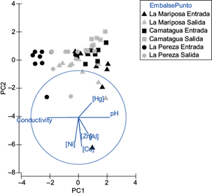
Fig. 2 Principal components analysis for water samples. PC1 represents pH and conductivity. PC2 represents Cu and Ni concentrations. Both principal components represent 55.5 % of variance.
Median concentration of metals in water are in table II, where it can be observed that the decreasing order in LM was [Al] ˃ [Cu] ˃ [Zn] ˃ [Ni] ˃ [Hg], CM [Cu] ˃ [Zn] ˃ [Ni] ˃ [Hg] and LP [Zn] = [Ni] ˃ [Cu] ˃ [Hg]. Median concentrations of some metals in water were above EPA and Decree 883 guidelines (Table II).
TABLE II RANGE AND MEDIAN ± STANDARD DEVIATION OF METALS CONCENTRATIONS IN WATER SAMPLES (PPM).
| Reservoir | Sampling point | Al | Zn | Ni | Cu | Hg (ppb) |
| La Mariposa | Entrance | 0.9 ± 2 | 0.2 ± 0.3 | 0.2 ± 0.6 | 0.3 ± 0.6 | 0.1 ± 0.1 |
| 0 - 4.3 | 0 - 0.8 | 0 - 1.8 | 0 - 1.8 | 0 - 0.4 | ||
| Exit | 0.6 ± 2 | 0.4 ± 0.5 | 0.04 ± 0.08 | 0.4 ± 0.1 | 0.1 ± 0.1 | |
| 0 - 5.8 | 0 - 1.1 | 0 - 0.3 | 0.2 - 0.7 | 0 - 0.3 | ||
| Camatagua | Entrance | ˂LD(c) | ˂LD(c) | 0.2 ± 0.3 | 0.03 ± 0.07 | 1 ± 2 |
| 0 - 0.9 | 0 - 0.2 | 0 - 6 | ||||
| Exit | ˂LD(c) | 1.2 ± 0.9 | 0.3 ± 0.5 | 0.1 ± 0.08 | 3 ± 3 | |
| 0 - 2.4 | 0 - 1.5 | 0 - 0.2 | 0.1 - 8 | |||
| La Pereza | Entrance | ˂LD(c) | 0.04 ± 0.1 | 0.3 ± 0.7 | 0.1 ± 0.1 | ˂LD(c) |
| 0 - 0.3 | 0 - 2.1 | 0 - 0.2 | ||||
| Exit | ˂LD(c) | 0.5 ± 1 | 0.1 ± 0.2 | 0.06 ± 0.1 | 0.03 ± 0.06 | |
| 0 - 3 | 0 - 0.5 | 0 - 0.2 | 0 - 0.1 | |||
| EPA(a) | 0.75 | 0.12 | 0.47 | 0.013 | 1.4 | |
| Decree No 883(b) | 0.2 | 5 | 1 | 10 |
*a)EPA guidelines, 2002. EPA-822-R-02-047.
*b) Decree No 883, (1995) guidelines for waters subtype 1A and 1B.
*c) Below detection limit.
Linear regression analysis with the metal concentration in water was not related to any of the environmental variables measured (pH, conductivity, metal concentration in sediments, and bioavailable fraction).
Sediments
Metals concentration in sediments were different between reservoirs (pperm=0.001; Fig. 3). Additionally, using the Monte Carlo test, the sediments metal concentration was significantly different between sampling points (entrance and exit) of LM and LP (MC = 0.001; Fig. 3). Sampling points in Camatagua had no significant differences between the entrance and exit sample points; however, the exit point had the highest OM, TOC, and Hg concentrations. The relationship between metals concentration in sediments with pH and conductivity was significant for Zn, Ni, Hg, and Al with pH (p ˂ 0.03) and Hg and Al with conductivity (p ˂ 0.01; Fig. 3). The highest metal concentration was LMs’ sediment samples, followed by LP and last CM.
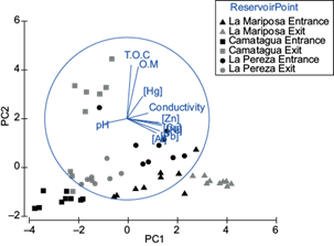
Fig. 3 Principal components analysis for sediment samples. PC1 represents the metal concentration of Pb, Al, Zn, Ni, and Cu. PC2 represents TOC and O. Both principal components represent 71 % of the variance.
The median concentration of metals in sediments in LM was in decreasing order: [Al] ˃ [Zn] ˃ [Cu] ˃ [Ni] ˃ [Pb] ˃ [Hg]; CM [Al] ˃ [Zn] ˃ [Cu] ˃ [Ni] ˃ [Pb] ˃ [Hg] and LP [Al] ˃ [Zn] ˃ [Cu] ˃ [Ni] ˃ [Pb] ˃ [Hg]. Median concentrations of some metals in sediments were above EPA, Dutch and Canada guidelines (Table III).
TABLE III RANGE AND MEDIAN ± STANDARD DEVIATION OF METALS CONCENTRATIONS IN SEDIMENT SAMPLES (PPM DRY WEIGHT).
| Reservoir | Sampling point | Pb | Al | Zn | Ni | Cu | Hg |
| La Mariposa | Entrance | 40 ± 10 | 50000 ± 20000 | 70 ± 40 | 50 ± 10 | 70 ± 20 | 0.08 ± 0.03 |
| 18 - 60 | 26147 - 69711 | 33 - 143 | 31 - 73 | 35 - 97 | 0.04 - 0.1 | ||
| Exit | 70 ± 8 | 40000 ± 10000 | 200 ± 30 | 70 ± 10 | 100 ± 10 | 0.10 ± 0.01 | |
| 54 - 81 | 24087 - 67013 | 177 - 268 | 61 - 93 | 97 - 131 | 0.09 - 0.1 | ||
| Camatagua | Entrance | 1 ± 2 | 900 ± 500 | 30 ± 10 | 3 ± 2 | 6 ± 4 | 0.012 ± 0.005 |
| 0 - 6 | 354 - 1692 | 10 - 53 | 0.8 - 6 | 1 - 11 | 0.004 - 0.02 | ||
| Exit | 7 ± 5 | 1300 ± 500 | 50 ± 20 | 8 ± 4 | 17 ± 6 | 0.1 ± 0.06 | |
| 0 - 15 | 658 - 2281 | 31 - 89 | 4 - 13 | 9 - 30 | 0.02 - 0.2 | ||
| La Pereza | Entrance | 20 ± 7 | 3300 ± 1000 | 100 ± 50 | 50 ± 20 | 60 ± 30 | 0.1 ± 0.1 |
| 0 - 24 | 11 - 4688 | 0.4 - 167 | 0 - 82 | 0 - 87 | 0.02 - 0.2 | ||
| Exit | 8 ± 6 | 2000 ± 800 | 70 ± 30 | 10 ± 3 | 30 ± 9 | 0.05 ± 0.04 | |
| 0 - 19 | 817 - 3220 | 39 - 118 | 8 - 18 | 16 - 46 | 0.02 - 0.2 | ||
| EPA(a) | 37 | 98 | 19.514 | 28.012 | |||
| Dutchland(b) | 50 | 140 | 30 | 40 | 0.15 | ||
| Canada(c) | 35 | 123 | 35.7 | 0.17 | |||
| Peru(d) | 140 | 6.6 |
*a)EPA, 1996. (ARCS) guidelines. EPA-905-R96-008.
*b) Dutch law guidelines for environmental management, 2008. Baseline values.
*c)Canadian guidelines for sediment quality for aquatic wildlife protection, 1999. ISQG.
*d) Peru guidelines for environmental quality (ECA) for soils, 2017. Residential soils / parks.
LM’s sediments had an EF between 5-20, and according to Sutherland’s (2000) classification, it indicates significant contamination in this water reservoir. However, LP and CM had an EF ˂ 2, suggesting minimal or no contamination as specified by Sutherland (2000).
Bioavailable fraction
Pb was detected only in three samples of the bioavailable fraction, two from LP (2.14 and 1.72 ppm) and one from LM (4.9 ppm). There were significant differences between reservoirs (pperm = 0.001; Fig. 4) and between sampling points (entrance and exit) of LM and LP (MC = 0.018 and 0.005, respectively; Fig. 4). The highest metal concentrations were LPs’ bioavailable fraction samples, follow by LM and CM. Except for Hg, which had higher concentrations in CMs’ bioavailable fraction samples. In figure 4 is a pattern where metal concentration in the bioavailable fraction increases with conductivity and lower pH. These relations were especially significant between Zn, Ni, and Cu (p ˂ 0.01).
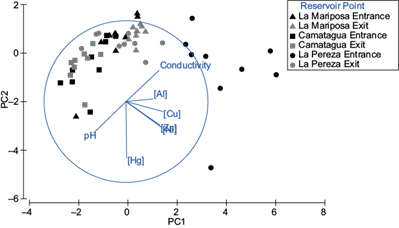
Fig. 4 Principal component analysis for bioavailable fraction of sediments. PC1 represents Pb, Al, Zn, Ni and Cu concentrations, pH, and conductivity. PC2 represents Hg concentrations. Both principal components represent 78.2 % of variance.
Mean concentrations of metals in bioavailable fraction are in table IV, the decreasing order in LM’s entrance was [Al] ˃ [Cu] = [Ni] ˃ [Zn] ˃ [Hg]; LM´s exit [Al] ˃ [Cu] ˃ [Zn] = [Ni] ˃ [Hg]; CM [Al] ˃ [Zn] ˃ [Ni] ˃ [Cu] ˃ [Hg]; LP´s entrance [Al] ˃ [Zn] ˃ [Ni] ˃ [Cu] ˃ [Hg] and LP´s exit [Zn] ˃ [Al] ˃ [Cu] ˃ [Ni] ˃ [Hg]. On the other hand, LP had an SQGQ ˃ 1, suggesting a toxicology risk for the mix of contaminants assessed, contrary to LM and CM´s bioavailable fraction, which had an SQGQ ˂ 1 (Fairey et al. 2001).
TABLE IV RANGE AND MEDIAN ± STANDARD DEVIATION OF METALS CONCENTRATIONS IN BIOAVAILABLE FRACTION OF SEDIMENT SAMPLES (PPM DRY WEIGH).
| Reservoir | Sampling point | Al | Zn | Ni | Cu | Hg (ppb) |
| La Mariposa | Entrance | 90 ± 30 | 1 ± 1 | 5 ± 1 | 5 ± 2 | 4 ± 9 |
| 64 - 140 | 0 - 3 | 3 - 7 | 3 - 8 | 0 - 28 | ||
| Exit | 200 ± 30 | 4 ± 2 | 4 ± 1 | 8 ± 1 | 4 ± 3 | |
| 142 - 230 | 2 - 10 | 2 - 4 | 6 - 9 | 0.4 - 11 | ||
| Camatagua | Entrance | 40 ± 20 | 10 ± 3 | 2 ± 0,8 | 2 ± 0,9 | 10 ± 10 |
| 21 - 83 | 7 - 15 | 1 - 4 | 0.5 - 3 | 0 - 40 | ||
| Exit | 10 ± 20 | 20 ± 9 | 3 ± 1 | 0.4 ± 0.7 | 10 ± 10 | |
| 0 - 47 | 8 - 40 | 2 - 4 | 0 - 2 | 0.2 - 28 | ||
| La Pereza | Entrance | 150 ± 70 | 170 ± 60 | 60 ± 20 | 30 ± 10 | 10 ± 20 |
| 63 - 276 | 83 - 241 | 31 - 89 | 15 - 42 | 0 - 63 | ||
| Exit | 20 ± 30 | 40 ± 40 | 8 ± 6 | 8 ± 7 | 2 ± 2 | |
| 0 - 76 | 0 - 136 | 0 - 15 | 0 - 23 | 0 - 7 |
Eichhornia crassipes
The bioconcentration factor of E. crassipes had significant differences between organs (pperm=0.005; Fig. 5) and reservoirs (pperm=0.049; Fig. 5), being the highest sources of variation. Differences between sampling points were not assessed due to an imbalance in sampling. In figure 5 is appreciated that the highest concentrations of metals in E. crassipes were LMs’ samples, except for Hg, which was more abundant in the CM (Fig. 5). On the other hand, roots had higher concentrations of Pb, Al, Ni, and Hg, while leaves had higher concentrations of Zn and Cu.

Fig. 5 (a) Principal components analysis for bioconcentration factor of E. crassipes. PC1 represents Cu and Al concentrations. PC2 represents Ni concentrations. Both principal components represent 78.5 % of variance. (b) Principal components analysis for bioconcentration factor of L. minor. PC1 represents Cu, Zn and Al concentrations. PC2 represents Hg concentrations. Both principal components represent 72.9 % of variance.
Differences between leaf and root of E. crassipes are in figure 6. Pb was found only in the roots. Ni, Hg, and Al were more abundant in the roots, and Al was present only in the leaves of LM. Zn and Cu were more abundant in LMs’ leaves. Similar to CM, where Zn was more abundant in leaves, but Cu was more abundant in roots.
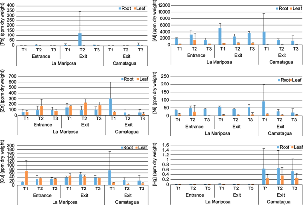
Fig. 6 Mean concentration and standard deviation of metals in roots and leaves of E. crassipes. (a) Pb, (b) Al, (c) Zn, (d) Ni, (e) Cu, and (f) Hg concentrations by transect and reservoir.
The decreasing order of metals in E. crassipes roots of LMs’ samples were [Al] ˃ [Zn] ˃ [Ni] ˃ [Cu] ˃ [Pb] ˃ [Hg] and in leaves [Al] ˃ [Zn] ˃ [Cu] ˃ [Ni] ˃ [Hg]. CM had a similar pattern, the decreasing order in roots was [Al] ˃ [Zn] ˃ [Ni] ˃ [Cu] ˃ [Pb] ˃ [Hg] and in leaves [Zn] ˃ [Cu] ˃ [Ni] ˃ [Hg]. There were significant relations between Al (root), Cu (root) and Zn (leaves) concentrations with metal concentration in sediments and bioavailable fraction (p ˂ 0.04). These relations were only significant in E. crassipes samples from LM.
Lemna minor
There were no significant differences between organs in L. minor (Fig. 7) but there were between reservoirs (MC=0.035; Fig. 7), being this the highest source of variation. Ni, Al, Cu, and Zn were more abundant in LM. Mean concentration of metals in L. minor is in table V, the decreasing order of metals in LM was [Al] ˃ [Zn] ˃ [Cu] ˃ [Pb] ˃ [Ni] ˃ [Hg] and LP [Zn] ˃ [Cu] = [Al] ˃ [Cu] ˃ [Ni] ˃ [Pb] ˃ [Hg].
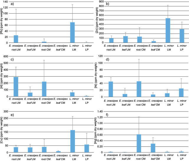
Fig. 7 Metals concentration in roots and leaves of E. crassipes and L. minor in three water reservoirs, La Mariposa (LM), Camatagua (CM), and La Pereza (LP). Bars represent the mean concentration with their corresponding standard deviation of Pb (a), Zn (b), Al (c), Ni (d), Cu (e), and Hg (f).
TABLE V RANGE AND MEDIAN ± STANDARD DEVIATION OF METALS CONCENTRATIONS IN L. minor (PPM DRY WEIGH).
| Reservoir | Pb | Al | Zn | Ni | Cu | Hg |
| La Mariposa | 70 ± 60 | 600 ± 300 | 500 ± 300 | 10 ± 10 | 200 ± 100 | 0.02 ± 0.03 |
| 0 - 191 | 246 - 1274 | 209 - 1116 | 0 - 30 | 68 - 477 | 0.006 - 0.1 | |
| La Pereza | 1 ± 2 | 60 ± 100 | 300 ± 200 | 20 ± 30 | 60 ± 80 | 0.02 ± 0.03 |
| 0 - 6 | 0 - 374 | 0 - 697 | 0 - 100 | 0 - 303 | 0 - 0.1 |
There were significant relations between Al concentrations in L. minor with sediments and water concentrations (p ˂ 0.01). E. crassipes and L. minor samples could not be compared due to unbalanced sampling. However, L. minor had the highest Pb concentrations in LM (Fig. 8). Al was more abundant in E. crassipes, contrary to Zn and Cu which had higher concentrations in L. minor. Ni concentrations were similar among L. minor and E. crassipes leaves, and Hg was more abundant in CMs’ plants.
DISCUSSION
La Mariposa (LM), Camatagua (CM), and La Pereza (LP) reservoirs had significant differences in metal content in all compartments analyzed, being the highest source of variation. Despite the importance of these water bodies, this has not been studied before. LM and LPs’ water samples had the highest metal concentrations; this could be related to the discharges rich in organic matter from farmhouses, pig houses, and informal houses located in the slopes of these reservoirs (González and Ortaz 1998, González et al. 2003, Bentancourt and Mena 2012). The water waste of these sources tends to be rich in metals like Cu, Ni, and Zn (Sutherland 2000). On the other hand, LM had high concentrations of Pb; a possible origin could be antiknocks of gasoline, before the abolition of its use in 2000 decade; other sources could be wastes from industries, mining, and smelters (Kabata-Pendias 2010). Although, the last ones have not been reported in previous works. Additionally, pointing a specific cause of metals pollution is hard, and it should be addressed in new projects. Unlike LM and LP, CM was the least intervened. This is one of the largest reservoirs of the country, and despite receiving water from contaminated sources such as the Guarico river it also receives from non-contaminated sources (Meléndez et al. 2006).
Zn, Ni, Cu, and Hg concentrations in water of the three reservoirs were higher than those reported for the Zuata reservoir, Aragua state, Venezuela (Álvarez et al. 2012). However, Pb concentrations in water samples from Zuata were higher than in LM, CM, and LP. There were no differences in water samples between sampling points in the three reservoirs, this could be due to water currents in the surface, a product of wind and convection movements by the gradient between day and night (Lewis 1983). On the other hand, despite the regression analysis not being significant, it has been reported that pH and total suspended solids have a relation with the metal concentration in water (Eggleton and Thomas 2004).
LM and LPs’ sediments had significant differences between sampling points, this could be due to differences in deep sampling. A deeper sample could have a higher content of metals due to sulfide production (Zhang et al. 2014). On the other hand, these differences could also be related to variables like organic matter, TOC, and pH (Kabata-Pendias 2010, Zhang et al. 2014), which were significantly related to the metal concentration in sediments.
Metal concentration in sediments of the three reservoirs was lower than the reported for the Zuata reservoir, except for Pb, which was higher in LM’s sediments (Álvarez et al. 2012). On the other hand, metal concentration in sediments of the three reservoirs surpassed some international guidelines. Additionally, according to Sutherland (2000) classification, LM’s sediments have significant contamination. Unlike CM and LP, which have minimum contamination also according to Sutherland (2000) classification.
The bioavailable fraction of LP had the highest metal concentration, despite LMs’ sediments having the highest metal concentration. These differences could be related to the acid pH of LP, which could increase the solubility and mobility of metals like Zn and Ni (Zhang et al. 2014). Nonetheless, other variables can affect the observed pattern, like clay percentage and origin and nature of the metal (Eggleton and Thomas 2004). On the other hand, according to the toxicology index, LP’s bioavailable fraction could be a toxicology risk to microorganisms (Fairey et al. 2001). Additionally, the fish consumed by locals in LM reservoir could have high concentrations of metal in tissue, being a potential risk for humans. Moreover, this is one of the first studies of this type. However, future studies in risk assessment are needed.
Pb concentrations in bioavailable fraction were below the detection limit, this could be due to its nature. Pb tends to be adsorbed in organic matter and clay, reducing its solubility and mobility (Eggleton and Thomas 2004). Ni and Zn were the most common elements in this compartment, following literature. Likewise, Cu in LM’s bioavailable fraction was among the most common metals, this could be due to its origin. Cu from anthropic input is more mobile and soluble than compounds with lithological origin (Kabata-Pendias 2010).
The highest concentrations of Hg in sediments were in LM and LP samples. However, the water and the bioavailable fraction of CM had the highest concentrations of this metal. This pattern could be related to the aerobic conditions of the reservoir. The bioavailability of Hg in water systems is highly dependent on the methylation rates, which in turn is related to the oxygen levels (Boszke et al. 2008). In anoxic systems, anions of Hg are bound to sulfides and are less available, contrary to aerobic ecosystems, where the formation of cations that can participate in the methylation process is favored (Boszke et al. 2008, Kabata-Pendias 2010). According to González et al. (2003), and González and Roldán (2019) the three reservoirs studied are eutrophic due to the phosphorus and nitrogen ratio and phytoplankton biomass. However, the euthrophic conditions are less critical in CM (González and Roldán 2019). In other words, CM could have more oxygen availability, and in consequence favor the formation of more mobile forms of Hg than LP and LM (Boszke et al. 2008, Kabata-Pendias 2010).
There were differences in metal content between E. crassipes and L. minor according to the reservoir. This could be a reflection of environmental variables like organic matter, TOC, pH, and metal concentration (Lu et al. 2004, Bonanno and Giudice 2010). However, other variables could affect the observed pattern, like antagonistic relations between metals, root area, grain size, and genetic factors (Kabata-Pendias 2010). On the other hand, the differences between organs in E. crassipes have been reported in other studies, aquatic macrophytes like E. crassipes tend to have 5 - 60 times higher concentrations of metals in roots than in leaves (Quian et al. 1999, Soltan and Rashed 2003). However, Zn and Cu were more abundant in leaves. This could be attributed to their nature, both metals are micronutrients of plants, involved in different metabolic pathways (Lu et al. 2004). For that reason, the translocation to leaves depends on the metal concentration in the environment (Kabata-Pendias 2010), being favorable in sites like LM where Zn and Cu were abundant in the bioavailable fraction. However, other variables like metal mobility, phosphorous content, and ligands presence could affect the observed pattern (Hadad et al. 2009).
Unlike E. crassipes, there were no differences between organs in L. minor, opposed to Kastratovic et al. (2015) study. The investigators found differences between roots and leaves for Cd, Cu, Co, Cr, Mn, Ni, Pb, Zn, V, and Sr. These differences between studies could be consequences of L. minor size. Metals entrance in plants occurs in roots and leaves, in a small plant-like L. minor, metal ingress in both organs could be similar, leading to little differentiation between the two. However, other studies should be carried out with a larger sampling size to evaluate this hypothesis.
There were some differences between E. crassipes organs, where roots accumulated more metals than leaves. In consequence, the roots are better suited for bioindicator studies by accumulation. In the case of L. minor, there were no differences between organs, and metal content can be assessed in the whole body. On the other hand, E. crassipes and L. minor had some differences, which could be a consequence of genetic and physiological factors. Nonetheless, metal content in E. crassipes roots and L. minor had a similar pattern to water, sediments, and bioavailable fraction. Moreover, many of those relations were statistically significant. Overall, these patterns suggest that both plants are potential bioindicators for the three water reservoirs studied, especially for water and the bioavailable fraction of sediments. Lastly, since E. crassipes is a perennial plant (Rezania et al. 2016) its roots could reflect environmental quality for a longer period than L. minor. Which has a short period of life (15 days) and could reflect the momentary system conditions (Barks and Laird 2014).
CONCLUSIONS
This is the first study to evaluate the metal content in La Mariposa, Camatagua, and La Pereza reservoirs. There were significant differences between the three. Those differences are intimately related to environmental variables like organic matter, TOC, and pH. There were also differences between E. crassipes organs, where roots accumulated more metals than leaves. On the contrary, there were no differences between L. minor organs. The differences found between reservoirs are reflected in E. crassipes organs but are more clear in its roots. Likewise, these patterns were also clear in L. minor, suggesting that both plants have potential as bioindicators of metal contamination for some water reservoirs, where E. crassipes could reflect the environmental quality for a longer period than L. minor.

