text new page (beta)
 English (pdf)
 Article in xml format
 Article references
 Send this article by e-mail
 Cited by SciELO
  Similars in
SciELO
Similars in
SciELO 
 Permalink
INTRODUCTION
The need to combine the development of national defence with the conservation of natural values and quality of life in the vicinity of the Spanish Air Force’s air bases, requires a seires of measures based on the coordination of economic, social and environmental factors that allow us to approach a sustainable development model.
In particular, noise pollution is one of the main environmental aspects generated as a result of military activity. Hence, the minimization of noise levels and protection of population’s quality of life in the environment of military facilities has become one of the priorities of the Spanish Defence Ministry1.
Among the activities carried out in air bases, the main sources of noise emission are the operations of military aircraft taking off and landing, and, at a lower level, preflight preparations on runways. International, national and even regional regulations concerning airport facilities on noise pollution do not apply to the military in Spain2.
The measures implemented by the Spanish Air Force, designed to minimize the inconvenience caused by noise, comprises six key aspects: reducing noise at source; planning and management of land use, procedures and operations for noise abatement; restrictions on military aircraft operations; ongoing impact assessment produced; flows of communication and collaboration with local authorities, stakeholders and the general public; and implementation of plans for sound insulation.
As a general objective, we consider the depreciation of value of urban housing caused by the environmental impact of noise pollution emitted by military aircraft operating in the Gando Air Base, using the methodology of hedonic pricing, limiting our study to a specific geographical area covering three municipalities of the island of Gran Canaria (Telde, Agüimes and Ingenio) (Fig. 1).
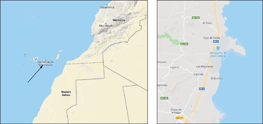
Google map.
There are several examples in the methodology of hedonic pricing. It has been used successfully by, for instance, Cohen and Coughlin (2008) where they analyze several econometric models to examine the impact of noise on a sample of 508 homes in 2003 near the airport of Hartsfield-Jackson in Atlanta (USA).
The result was that for homes that underwent between 70 and 75 decibels, their price decreased by 20.8 % in relation to homes that underwent less than 65 decibels.
Economists Jasper and Straaten (2009) used a logarithmic-linear model to study the effects of noise at the Amsterdam airport. For the 66 000 homes studied, the total benefit of decreasing noise by one decibel was 574 million euros.
Having presented and quantified levels of sound exposure in the study area through the strategic noise map, the data was summarized and variables or relevant aspects used in determinining urban household prices were analyzed in various national and international studies and econometric models were put together that best fitted our reality, including all variables previously selected and validated, with particular attention to environmental noise pollution variables.
Ultimately, this research invalidates the assumption “there are no effects of noise pollution from military aircraft over the selling price of homes in the study area”.
The main objective of this article is to study the attributes and implicit prices that best contribute to explaining the sale price of real estate in an airport area, by using the hedonic price method, considering environmental and noise pollution among the most relevant.
Subsequently, to present the model as a reference to be used, not only to explain the behavior of the price of homes adjacent to an airport, but which may also be used as a theoretical basis for drawing up future environmental policies for action and mitigation of noise pollution in airport environments, as well as predicting its behavior based on scenarios of occurrence regarding the explanatory variables included in the model.
MATERIALS AND METHODS
Background
It is increasingly common to find econometric studies using the hedonistic price method for the study of environmental problems, and in our case, for noise pollution in the real-estate market (Nelson 2004, Jasper and Straaten 2009).
Marmolejo and Romano (2009) took a step forward to explain that behind the willingness to pay, in the case of the Prat airport’s residential environment (Barcelona), there underlie different characteristic elements of real estate prices (proximity, type of housing, rent, etc.) through the aforementioned hedonic price method.
Adjusting hedonic price models to the case of housing has been a common exercise but has not been free from difficulties either due to data restriction or because of market heterogeneity. In the literature it is common to find cross-sectional studies in various markets (Schnare and Struyk 1976, Goodman 1988 or Hanley and Spash 1993). In the case of Spain, Bilbao (2000) or Bover and Velilla (2001), represent interesting examples.
Data collection
One feature of this analysis is that all impacts are measured in monetary units finally updated to 2012. That is, the prices of the houses studied correspond to the sale prices of that year (including taxes), using the methodology of cross-sectional data collection.
This study has been based on the strategic noise map drawn up in 2005 with data provided by the Gando Air Base itself and prepared by the National Institute of Aerospace Techniques Esteban Terradas (INTA).
The mapping used was obtained from the Air Force Centre for Mapping and Photogrammetry (CECAF). Additionally, we used the Electronic Office of the Directorate General of Land Registry to verify the different surface areas constructed and conservation status of affected households in the study area.
With respect to economic data regarding the market price of homes in the sample, information from various real estate websites (segundaman.com, fotocasa.es, elidealista.es and the Professional Association of Valuation Companies) and evaluations were obtained.
Furthermore, we used data gathered from the Noise Map Report for Major Spanish Airports for the civilian airport of Gran Canaria, which shares runways with military facilities (MINISFOM and AENA 2007).
The results of several relevant studies were used in assessing noise to calculate depreciation in the real estate market in the area (Commission on the Third London Airport and Roskill 1971, Rosen 1974), as well as a contrast study of the US Orange County Health Department regarding the reactions of the population to noise depending on perceived decibels (Randall 2001).
In these studies a series of datatables, transposed to Gran Canaria Airport data were used, and therefore the Gando Air Base by the similarities of both airports. Finally, for the econometric evidence of the different models of hedonic functions, the GRELT (Gnu Regressión, Econometric and Time Series) computer free program was used.
The sources considered in the face of computer modeling, pertain only to landing and takeoff operations of the Fockker 27 and the EF-18 Hornet with origin or destination in Gando Air Base because these two types of aircraft operate on the Air Base permanently and are the most responsible for acoustic pollution.
The INM (Integrated Noise Model) was used to calculate noise levels (FAA 1999). Previous considerations:
The total number of annual military operations considered is 6245 for 2005. Of total operations, 95 % were carried out by EF-18 Hornets. In addition, 98 % of daytime operations were carried out from 7:00 to 19:00 h).
The existing flight field for the calculation scenario consists of two parallel runways of asphalt concrete: 03L-21R and 03R-21L, both 3100 m long and 45 m wide. In the study, runway 03R-21L will be taken into account, as it practically has almost exclusively military use.
The position of the existing runways is based on the coordinates and altitude published in the AIP (Aeronautical Information Publication) corresponding to the Gran Canaria Airport.
The meteorological conditions in relation to the propagation of sound are standard temperature and humidity, standardized wind speed at the front end of 14.8 km/h, and without temperature variations with height.
Flat land around the Air Base, calculating attenuation due to land in accordance with SAE AIR 1751 (SAE 1981), adopted by European Civil Aviation Conference, and the noise maps are calculated for a height of 4 m above ground.
Based on the input data and the methodology described, the noise levels in the Air Base environment have been calculated for the two selected indices (Lnight and Lden). The results of sound impact, and in the absence of legislation that establishes the admissible limits of sound emmission, are shown by means of noise maps that represent noise levels caused by isophones of a sound level from 60 decibels (A) for L den, and from 50 decibels (A) for Lnight (Table I, Fig. 2 and Fig. 3).
TABLE I AREA AFFECTED BY HECTARES AND DECIBEL LEVEL (A) IN THE L den PERIOD
| Level (dBA) | Color | Area (ha) | Inside base | Out side base* | ||||
| ha | % | ha | % | |||||
| 60-65 | Green | 1050 | 514 | 49 | 544 | 51 | ||
| 65-70 | Blue | 440 | 256 | 60 | 184 | 40 | ||
| 70-75 | Orange | 180 | 180 | 100 | 0 | 0 | ||
| > 75 | Red | 200 | 200 | 100 | 0 | 0 | ||
(*)Only land area, we do not include the area that affects the sea


The following tables II and III, summarize the data obtained in relation to the sample studied.
TABLE II TYPOLOGY OF PREDOMINANT HOUSING BY MUNICIPALITY AND ISOPHONIC SCENARIO 2012
| Municipality/ Urban area | Predominant form of housing |
Population and housing census (2012) |
Isophonics | |||
| Single family | Block of flats | Population | Housing | dB(A) Lden |
Observations | |
| TELDE | 55-70 | |||||
| Taliarte | YES | YES | 366 | 122 | 55-60 | It is in that interval the French Lyceum “René Vernau” institute. |
| Tufia | YES | NO | 40 | 14 | 55-65 | Most homes are between 60 and 65 dB (A) and only a small part, between 55 and 60 dB (A). Possible increase in population due to the existence of urban land that could lead to a future acoustic problem and scattered housing. |
| Ojos de Garza | YES | NO | 2 935 | 978 | 60-70 | Population very concentrated on the coast, north of the runway, around 65 dB (A). |
| INGENIO | 55-70 | |||||
| Las Puntillas | YES | NO | 279 | 93 | 60-70 | The most exposed enclave since the 65-70 dB (A) range predominates, with some homes reaching more than 70 dB (A). |
| Las Majoreras | YES | YES | 1 844 | 614 | 55-70 | It presents greater variability in the type of housing, concentrating in 60 dB (A). |
| Carrizal | YES | YES | 12 606 | 4 202 | 55-60 | Greater population nucleus near the AB, however, only a small part is in the study area. Growth towards limited AB, not being contemplated in its planning and by the GC-1 highway. In addition, the Barrio Costa institute is located. Although it is not within the study area, the Carrizal institute is located very close to 55 dB (A). |
| El Burrero | YES | NO | 1 248 | 416 | 60-65 | Its development in the direction of the AB is not foreseen by the approved planning. |
| AGÜIMES | 55-70 | A large part of the affected area belongs to the Arinaga Industrial Estate, one of the most important industrial centers and free zones at state level. | ||||
| Urb. Paraíso | YES | NO | 56 | 20 | 60-70 | Despite not being the closest to the AB, it is aligned with the take-off and landing paths so that some homes are included in a range of between 65-70 dB (A). In the planning does not foresee the growth of this residential area. |
| Urb. Edén | YES | NO | 52 | 18 | 55-60 | |
| SANTA LUCIA DE TIRAJANA | NO | NO | - | - | 55-60 | There are no large nuclei, only scattered houses are present. Minimal involvement |
Compiled by authors based on data from the MINISFOM and AENA (2007). Strategic Noise Maps of Major Airports, Airport of Gran Canaria, Report May 2007
TABLE III INTERVALS OF LOSS OF VALUE EUROS / m2 ACCORDING TO URBAN AND ISOPHONIC NUCLEUS OF AFFECTATION AND RESPONSE OF THE POPULATION TO NOISE SCENARIO 2012
| Municipality | Isofhonics | Housing | Level dB(A) | Response population noise | |||||
| Intervals dB(A) L den | Housing Afectted | Acustic Isolation Plan | Price m2 | Intervals of loss of value Euros / m2 | L den> Acceptable Level *** | Public Response | |||
| TELDE | 55-70 | 112 | 1201.18 | ||||||
| Taliarte | 55-60 | 122 | 48.04 | 132.12 | 5 | sporadic complaints | |||
| Tufia | 55-65 | 14 | 144.14 | 204.20 | 10 | usual complaints | |||
| Ojos de Garza | 60-70 | 978 | 228.23 | 264.26 | 20 | strong complaints | |||
| INGENIO | 55-70 | 91 | 980.63 | ||||||
| Las Puntillas | 60-70 | 93 | 186.32 | 215.73 | 10 | usual complaints | |||
| Las Majoreras | 55-70 | 614 | 117.67 | 166.70 | 5 | sporadic complaints | |||
| Carrizal | 55-60 | 4202 | 39.22 | 107.87 | 5 | sporadic complaints | |||
| El Burrero | 60- 65 | 416 | 117.67 | 166.70 | 5 | sporadic complaints | |||
| AGÜIMES | 55-65 | 28 | 1225.40 | ||||||
| Urb. Paraíso | 60-70 | 20 | 232.82 | 269.58 | 10 | usual complaints | |||
| Urb. Edén | 55-60 | 18 | 49.01 | 134.79 | 5 | sporadic complaints | |||
| SANTA LUCIA DE TIRAJANA | 55-60 | - | 0 | 1027.00 | 10.27 | 30.81 | 10 | usual complaints | |
Data obtained from the National Statistics Institute street map of the different town halls, calculated according to the area affected according to the acoustic footprint reached in our study for the year 2012
Econometric estimation of the hedonic pricing function
Selection and classification of variables
Endogenous or dependent variable is the selling price of the property market for 2012 and the final sale prices in euros, including taxes. Given the clear market segmentation for housing (new or used, rental, subsidized housing, etc.) and to avoid distortions in the results, we only took into account the market sale price of homes over two years old, affected at different levels of noise pollution from military aircraft and geographically limited to the municipalities of Ingenio, Agüimes and Telde. In establishing the price transaction costs (taxes or fees) were not taken into account.
As table IV shows, the explanatory or exogenous variables are grouped by different attributes or dimensions of housing (Freeman et al. 2014).
TABLE IV EXPLANATORY OR EXOGENOUS VARIABLES BY HOUSING CHARACTERISTICS, DEFINITION AND EXPECTED SIGN
| Variables | Definition | Expected sign |
| Structural characteristics of housing | ||
| Builded surface (Scon) | Continuous variable in m2 total built in one, two or three floors for single family homes, apartment buildings and for multi-family housing. | Positive |
| Soil surface (Ssue) | Continuous variable field in which housing has been built, partly or wholly, in m2 which is part of the same the land register reference. | Positive |
| Old building (Antg) | Discrete variable referencing construction time in years for the property up to December 2012. | Negative |
| Housing typology (Tipo) | Dummy variable with value 1 if the housing is detached, and value 0 if it is not. | Indifferent |
| Conservation status (Econ) | Dummy variable depending on the general condition of the house (facade, finishing, quality materials, etc.): Very bad state (Econ1). Bad state (Econ2). Regular state (Econ3). Good state (Econ4). Very good state (Econ5). | Depending on the state of housing. |
| Noise protection measures (Mpac) | Dummy variable with value 1 if the house has windows or double glazing and shutters that isolate outside noise. | Positive |
| Passable roof (Atra) | Dummy variable equal to 1 for homes with roof and passable. | Indifferent |
| Availability garden, porch or terrace passable (Djpt) | Dummy variable equal to 1 for homes with accessible garden, porch or terrace passable. | Positive |
| Garage (Garj) | Dummy variable equal to 1 for houses with garage. | Positive |
| Number of rooms / bedrooms (Nhab) | Discrete variable that tells us the approximate number of rooms / bedrooms that home has. | Positive |
| Number of bathrooms / toilets (Nase) | Discrete variable that shows us the approximate number of bathrooms / toilets that the home has. | Positive |
| Socioeconomic and urban environment characteristics | ||
| Location (Locn) | Dummy variable with value 1 which reflects closeness to gardens, leisure and green areas, schools, hospitals / outpatient, day care centers and sports facilities. | Positive |
| Focus distance noise (Dist) | Continuous variable that expresses the distance in meters of runway 03R Gando Air Base, between the housing and the noise emitting source. | Indifferent |
| Communication and accessibility (Cyac) | Dummy variable equal to 1 if the housing is close (less than 1 km and unrestricted) public transport services, ease of access or roads in good condition as highways or freeways. | Positive |
| Geographic zone (Zgeo) | Dummy variable with value 1 depending on whether the sample belongs to the following municipalities: Ingenio (Zgeo1). Agüimes (Zgeo2). Telde (Zgeo3). | Indifferent |
| Level of complaints received (Nqpe) | Dummy variable with value 1 depending on the level of complaints received: No complaint (Nqpe1). Sporadic complaints (Nqpe2). Common complaints (Nqpe3). Considerable reaction (Nqpe4). Strong reaction (Nqpe5). | A higher level, a negative sign would be expected and vice versa |
| Environmental characteristic | ||
| Noise pollution (Cacu) | Dummy variable in decibels exposure Ldenin the area, divided into: Cacu1 Qi<55. Cacu2 55≤Qi<60. Cacu3 60≤Qi<65. Cacu4 65≤Qi<70. Cacu5 70≤Qi. | Depending on the level of perceived decibels |
Compiled by authors
Geographical limitation
For obtaining the simple random sample that we used on a study population of 6447 homes, we have made a division of two phases: assigning a number to each home and through random numbers generated by a computer, we chose as many subjects as necessary to complete the sample size3. Applying the selected data our sample size was 175 homes.
Model approach
Our econometric model has five initial environmental variables (Cocu1,…,5) depending on decibels perceived by each home. Economic theory does not clearly specify what is the best functional method (Freeman et al. 2014).
Furthermore, the selection of regressors takes evidence from multiple alternatives and comparisons. We should not forget that, if the chosen subject deals with a specific economic theory, it could help us to specify the model. Economic literature has established criteria for chooosing models.
The most commonly used criteria and implemented in this study are: maximization criterion adjusted determination coefficient (R2); Schwarz, Akaike and Hannan-Quinn Information Criteria; along with Ramsey Reset test to validate the functional form of the models shortlisted.
One of the simplest and most popular procedures, implemented in this study, is the stepwise backward regression consisting of a step-by-step selection of variables in the regression, based on a battery of sequential contrasts to decide procedure on regressors, one by one through a backward elimination of explanatory variables or regression, depending on the level of significance set to determine the region of acceptance or rejection of the null hypothesis.
This procedure excluded, one by one, on the basis of variables in the statistical model values of t-student. Finaly, we established five initial models proposed as a starting point the study. From these, different regression models and tests of global significance and information criteria were made (Table V).
TABLE V ESTIMATION RESULTS OF DIFFERENT MODELS
| Model | Value p F (K-1, N-K) | R2 | R2 adjusted | Residual sum of squares | Test ramsey reset | Information criteria | ||||||
| Statistic | Value p | AKAIKE | SCHWARZ | HANNAN-QUINN | ||||||||
| 1 | LIN - LIN | 9.41 e-59 | 0.883 | 0.865 | 2.59 e11 | 2.979 | 0.054 | 4239.48 | 4315.44 | 4270.29 | ||
| 2 | LOG - LIN | 4.87 e-51 | 0.852 | 0.829 | 8.897 | 37.262 | 7.55e-014 | 23.296 | 99.251 | 54.106 | ||
| 3 | SEMILOG | 5.07 e-75 | 0.941 | 0.929 | 3.523 | 0.424 | 0.656 | -126.820 | -31.877 | -88.309 | ||
| 4 | LIN - QUADRATIC | 1.12 e-54 | 0.887 | 0.864 | 2.51 e11 | 10.225 | 0.0001 | 4297.65 | 4,73.60 | 4328.46 | ||
| 5 | LOG - GENERAL | 9.52 e-73 | 0.947 | 0.934 | 3.150 | 1.289 | 0.279 | -134.431 | -20.499 | -88.217 | ||
Prepared by the authors based on the result of GRELT software
After analyzing the previous five models, we decided to choose model 5 as the most complete and the best fit, with the largest number of significant regressors (14) and which showed the best goodness of fit with correct flexible and functional form. Our model presents an endogenous variable logarithm, (20) constant linear variables including, (6) regressors in logarithms, (6) quadratically.
The model is overall significant because the result of the value p (f-statistic) is 9.52 e-73, well below 5 % so the null hypothesis is a generally accepted significant model. Regarding the coefficient of determination, it shows a very acceptable level and higher than previous models, that is, the value shows that exogenous variables explain 94.75 % of the dispersion of the endogenous variable so, initially, the goodness of fit is optimal.
The corrected determination coefficient with 93.42 % has the same interpretation. Finally, the Reset Ramsey test reports that the functional form is correct, the null hypothesis is always true considering a significance level of 5 %. The results of the values of endogenous squared and cubed are 0.156 and 0.146, respectively.
Model estimation and validation
Specification
Once a series of statistical tests and have been carried out and the explanatory variables with a higher coefficient have been eliminated, we decided to choose the final model (Table VI) where we maintain environmental variables (Cacu2,…4). The logarithm of selling price is the functional form that best fits the endogenous variable. All non-significant variables were removed individually with a level of significance below 0.05. Although, our goodness of fit is decreased compared with model 5, all regressors are significant at 5 %.
TABLE VI FINAL MODEL: ESTIMATION BY ORDINARY LEAST SQUARE, USING THE OBSERVATIONS 1-175. DEPENDENT VARIABLE: SALE PRICE OF THE DWELLINGS OF THE SAMPLE IN LOGARITHM
| Coefficient | Standard deviation | t-Statistical | p-Value | ||
| const | 10.360 | β 0 | 0.155 | 66.630 | <0.0001 |
| Scon | 0.003 | β 01 | 0.0003 | 10.908 | <0.0001 |
| Econ1 | -0.346 | β 0501 | 0.095 | -3.654 | 0.0003 |
| Econ2 | -0.231 | β 0502 | 0.074 | -3.125 | 0.0021 |
| Econ3 | -0.104 | β 0503 | 0.047 | -2.220 | 0.0278 |
| Garj | 0.136 | β 09 | 0.048 | 2.844 | 0.0050 |
| Nhab | 0.058 | β 10 | 0.017 | 3.431 | 0.0008 |
| Zgeo2 | -0.115 | β 1502 | 0.055 | -2.110 | 0.0364 |
| Cacu2 | 0.149 | β 1702 | 0.066 | 2.277 | 0.0241 |
| Cacu3 | 0.312 | β 1703 | 0.058 | 5.396 | <0.0001 |
| Cacu4 | 0.276 | β 1704 | 0.064 | 4.274 | 0.0003 |
| logSsue | 0.109 | β 19 | 0.033 | 3.330 | 0.0011 |
| sq_Antg | -2.67 e-05 | β 26 | 1.22 e-05 | -2.191 | 0.0299 |
| sq_Dist | 1.3020 e-08 | β 29 | 2.3323 e-09 | 5.5826 | <0.0001 |
| Mean of dependent variable | 12.072 | Standard deviation of dep. var. | 0.587 |
| Sum of squared residuals | 10.038 | Standard error of residuals | 0.250 |
| F-statistic (13. 161) | 61.608 | Value p (F) | 1.56 e-55 |
| Unadjusted R-squared | 0.833 | Adjusted R-squared | 0.819 |
| Log-likelihood | 1.800 | Akaike Criteria | 24.400 |
| Schwarz criteria | 68.707 | Hannan-Quinn criteria | 2.372 |
Prepared by the authors based on the result of Grelt software
Outliers
To detect the existence of outliers or influential observations in the model, we must make the contrast of standardized residuals (Fig. 4). Then, we can compare them with the critical reference interval of a distribution N (0,1), considered in this case in an interval (2,-2).
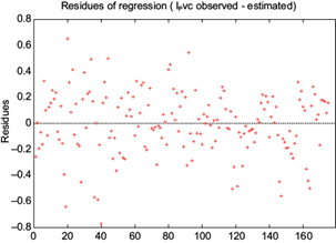
Fig. 4 Residuals model estimated for the sale price of the homes of the sample in logarithm.175 Observations
Depending on the interval chosen, there is no significant presence of outliers. There are a number of points of leverage, observations 4, 19, 36, 45, 46, 47, 78, 102, 105, 108, 109 and 123. These atypical individuals whose errors are abnormally high may have a potential or actual influence to substantially modify the regression plane, that is, the estimated model parameters. To check this, observations 4, 102, 105 and 123, would have a potential risk but not a certain influence.
Normality of disturbances
Specifically, we will analyze the graph of the frequency distribution (histogram) of the values of residuals (Fig. 5). At this point we compare the shape of this distribution that theoretically has the normal distribution, which would be unimodal, symmetrical and certainly flared.

To study the normality of the residuals of the estimated model, at first, we might consider the normal statistic that GRELT gives us by default, and this is the approach proposed by Doornik-Hansen (2008), contrast with a Chi-square with 2 degrees of freedom. We note a probability of 0.1194 for a Chi-square with 2 degrees of freedom (5.99) of 4.251, being in the region of acceptance, so we accept the null hypothesis, that is to say, disturbances are distributed normally.
Another interesting statistic is the statistic normality Jarque Bera (1980), based on the coefficients of skewness and kurtosis of the residuals of the regression, where the asymmetry coefficient (- 0.358) and kurtosis (0.424) approach 0 and 3 respectively, the probability of normality of the residuals by the result of lower index value Jarque Bera increases. With a value of 5.056 for a Chi-square with 2 degrees of freedom (5.99) and a probability p of 0.080, we would accept the null hypothesis of normality of residuals, reinforcing the idea that there is statistically significant evidence to reject the normality of residuals.
Goodness of fit and overall significance of the model
The model is globally significant because the result of p (F-statistic) is 1.56 e-55, well below 5 % so that the null hypothesis is accepted. In addition, the unadjusted R2 is still very acceptable. Exogenous variables explain 83.26 % of the dispersion of the endogenous variable, so in principle, the goodness of fit is good. The ajusted 2 has the same interpretation with 81.91 %. In short, there are variables that have not been taken into account in our model and its effects are embedded in the error term, so to explain the minimum remaining proportion of the total endogenous variability.
Functional form and structural change
To achieve this goal, we will have a comparison of nonlinearity (square) where acceptance of the null hypothesis shows that the relationship is linear. R2 0.355 obtained is also the test statistic: TR2 is equal to 62.181 with a p-value equal to 4.301 e-12 for a Chi-square with 2 degrees of freedom. With these results, we confirmed a linear relationship, so the linear functional form is correct. Additionally, to confirm that the relationship between variables is linear, we used the Ramsey Reset test. For our model, the functional form chosen is correct, with a probability of 1.51 e-11 and a statistic F (2.159) of 29.265 including quadratic and cubic terms, falling in the region of acceptance of null hypothesis. Moreover, the value of the endogenous variable squared and cubed is not significant at 0.652 and 0.812 of probabilities, respectively. Therefore, its functional form is correct, that is, it is a log-lin a model with logarithmic regression and 2 four-square regressors.
With regard to structural change, we could assume that there could be a structural change in the type of housing or geographical area, therefore we must test the stability within the (intra-sample) showing the parameters of our relationship and therefore, we divide the total sample into two subsamples of about the same size, n1 and n2, as was done in the Chow test from observation 88 with the following information: F (13, 148) equals 1.500, p value 0.123. As the statistic is lower than the value in the table test, the conclusion is that the null hypothesis is accepted and there is no structural change.
Heteroscedasticity and autocorrelation
First we graphically analyze of residuals (Fig. 6), representing absolute errors in the ordinate axis on endogenous on the abscissa and on the other hand, the squared errors in the ordinate axis on the explanatory nondichotomous variables of our model (Scon, logSsue, sqAntg and sqDist) on the horizontal axis.

In figure 6 we can see a linear fit between residuals and endogenous variable as we increase the price of housing. In addition, a number of outliers can be seen in the graph because they are far from the average values. Using the graph to check squared residuals against each of the exogenous values, none of the graphs show a clear relationship between the exogenous variables and squared residuals and between the endogenous variable and residues in absolute values.
But we can not rely only on a graphical analysis to find out whether the model is not homoscedastic. We have to carry out several analytical tests. Breusch-Pagan test (Greene 1998) uses the residuals obtained from the original regression, squaring and presents against independent variables. It is distributed as a Chi-square with p-1 degrees of freedom where p is the number of regressors in the auxiliary regression, which in our case is 13 without the constant. Its statistic would be the sum of the squared residuals, 31.343, between two, resulting in 15.671, with a p value of 0.267. The test statistic yields a value lower than the Chi-squared value with 13 degrees of freedom, which is 22.4. Thus we would accept the null hypothesis so that the result tells us that our model is homoscedastic.
Multicollinearity
After analyzing the correlation matrix between different exogenous variables of the model, the results obtained show no signs of multicollinearity, as there is no component with a value greater than 0.8. The correlation coefficients are reduced, being the highest numerically (0.778), the number of rooms/bedrooms (Nhab). To reinforce this idea and confirm non-multicollinearity, we analyzed auxiliary regressions, using each of the exogenous variables as an endogenous function of other explanatory variables in order to analyze their coefficient of determination and the inflation factor variance. As a result of having very low variance in the correlation matrix, the model can be used both for prediction, and for structural analysis.
RESULTS AND CONCLUSIONS
The estimated parameters of the hedonic price model are important to inform policy makers. Based on statistical tests shown above, it may be concluded that the hedonic price model proposed reasonably explains the behavior of the endogenous variable and therefore may be used to make predictions regarding the performance of this variable.
In estimating the model, the parameter values represent an indicator of significant importance in explaining the issue under study because on this basis, the form and degree of influence of each explanatory variable is determined.
According to the results of the estimates and considering the rest of the coefficients of the variables under ceteris paribus study, we will highlight the environmental variables, where the coefficient β 1702 indicates that for households that are affected by noise pollution from 55-60 decibels, their value is 16.11 % higher than other homes suffering other levels of noise pollution.
The β 1703 tells us that for households affected by noise pollution from between 60 to 65 decibels, their value is 36.65 % higher than other homes suffering other levels of noise pollution. And lastly, the coefficient β 1704 tells us that for households affected by noise pollution from 65-70 decibels, their value is 31.76 % higher than other homes suffering other levels of noise pollution.
The price of homes that are affected by a noise level between 55 and 60 decibels is 14.9 % more expensive than noise free and the highest noise level (more than 70 decibels). The price of homes that support a noise level between 60 and 65 decibels is 31.2 % higher than noise free and the highest noise level and 16.3 % higher than those seen affected by a noise level between 55 and 60 decibels.
The price of homes that withstand a noise level between 65 and 70 decibels is 27.9 % higher than noise free and the highest noise level, 13 % higher than those that are are affected by a noise level between 55 and 60 decibels and 3.3 % lower than those that support a noise level between 60 and 65 decibels.
A plausible explanation for these data is that if they suffer high decibel rates, the value of housing increases, because they are the most luxurious, nearest to the airport, in addition to large green areas and good communication, access and security of public transport.
Another way of applying the model is to obtain how much you can vary the endogenous variable if, for example, we had a house of 100 m2 built; 150 m2; 10 years old; with a garage; 2 rooms/bedrooms; located in the municipality of Ingenio; a middling state of preservation; at 1250 m from the airport and undergoing 65 to 70 decibels, leaving the rest of exogenous variables ceteris paribus.
The result would be a value equal to 11.614 logPvci (the sale price of homes in logarithms), that is, the sale price of homes in this case, is 110 697.05 euros.
We should mention that proper adjustment was achieved between prices and attributes of the dwellings. We obtained the really explanatory variables of price differences between properties and, their implicit marginal prices.
The choice of the appropriate functional form in our hedonic regression estimate was reduced to an empirical question, as there were no contributions in previous studies that demonstrate categorically that a particular functional form is the most suitable. Therefore, we must choose the one that best fits the data of the sample and the selected regressors.
In our case, the methodology of multiple regression by ordinary least squares concludes that the best approach is the semilog hedonic price model, using the price of as endogenous and in housing in logarithmic terms and as regressors: built surface; very poor state, poor or regular maintenance; the existence of a garage; number of rooms/bedrooms; noise pollution from 55 to 60, 60 to 65 and 65 to 70 decibels; logarithm of land surface; age squared; and distance to noise focus squared.
This result leads us to think that the studio isolated variable noise pollution, as the only relevant factor for our endogenous conclusions, is not conclusive and we need to add other explanatory variables that have a significant influence.
The fact that a property is near a noise source is not in itself conclusive evidence of a loss of real estate value. Therefore, the analyst must find and use valid methods to accurately measure the loss of the property at market value.
Consequently, airport noise pollution generated by Gando Air Base does not constitute a negative attribute for homes in the area, except in the case of noise levels above 70 decibels.
The prices of housing in the area have not been affected by this problem or by the distance to the noise source, which may explain why no housing or environmental policy measures have been taken either by the affected municipalities or by the Cabildo Insular de Gran Canaria or by the Government of the Canary Islands due to the noise of military aircraft.
If this can become a problem in the future, it will be a question of research that can be carried out with more recent data on prices and housing characteristics. Of course, our model is not able to answer if noise pollution is a factor influencing other dimensions of human welfare, wich could recommend the introduction of policies. This is, of course, out of the scope of our research.